| Contents [0/13] |
| 1 [1/13] |
| 2 [2/13] |
| 3 [3/13] |
| 4 [4/13] |
| 5 [5/13] |
| 6 [6/13] |
| 7 [7/13] |
| 8 [8/13] |
| 9 [9/13] |
| 10 [10/13] |
| 11 [11/13] |
| 12 [12/13] |
| 13 [13/13] |
| 1 [1/13] |
Figure 1.3: The compilation system.
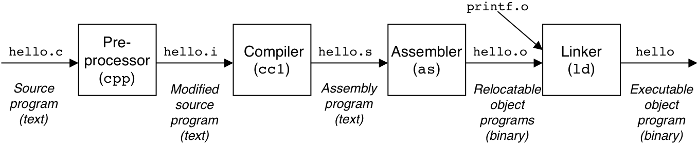
Figure 1.4: Hardware organization of a typical system.
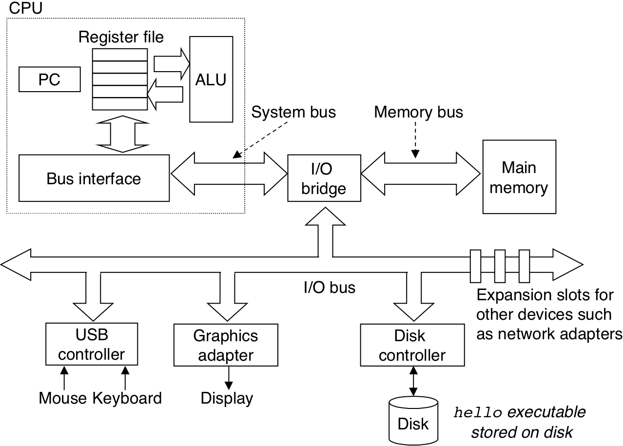
Figure 1.5: Reading the hello command from the keyboard.
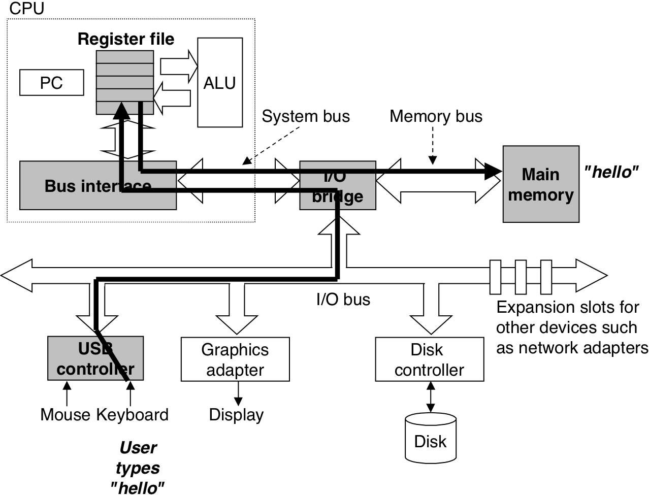
Figure 1.6: Loading the executable from disk into main memory.
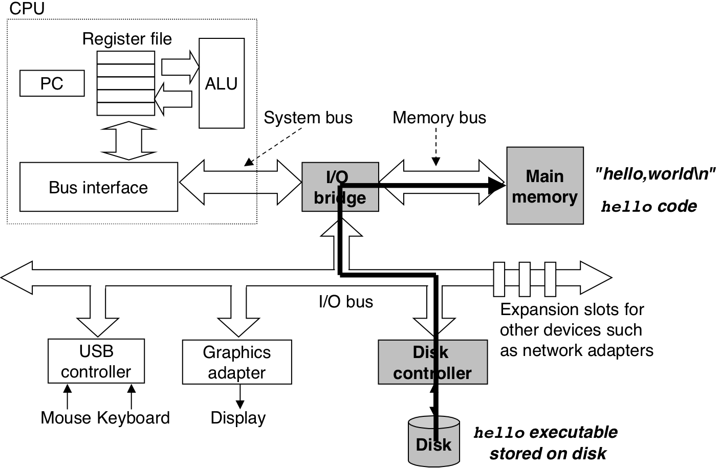
Figure 1.7: Writing the output string from memory to the display.
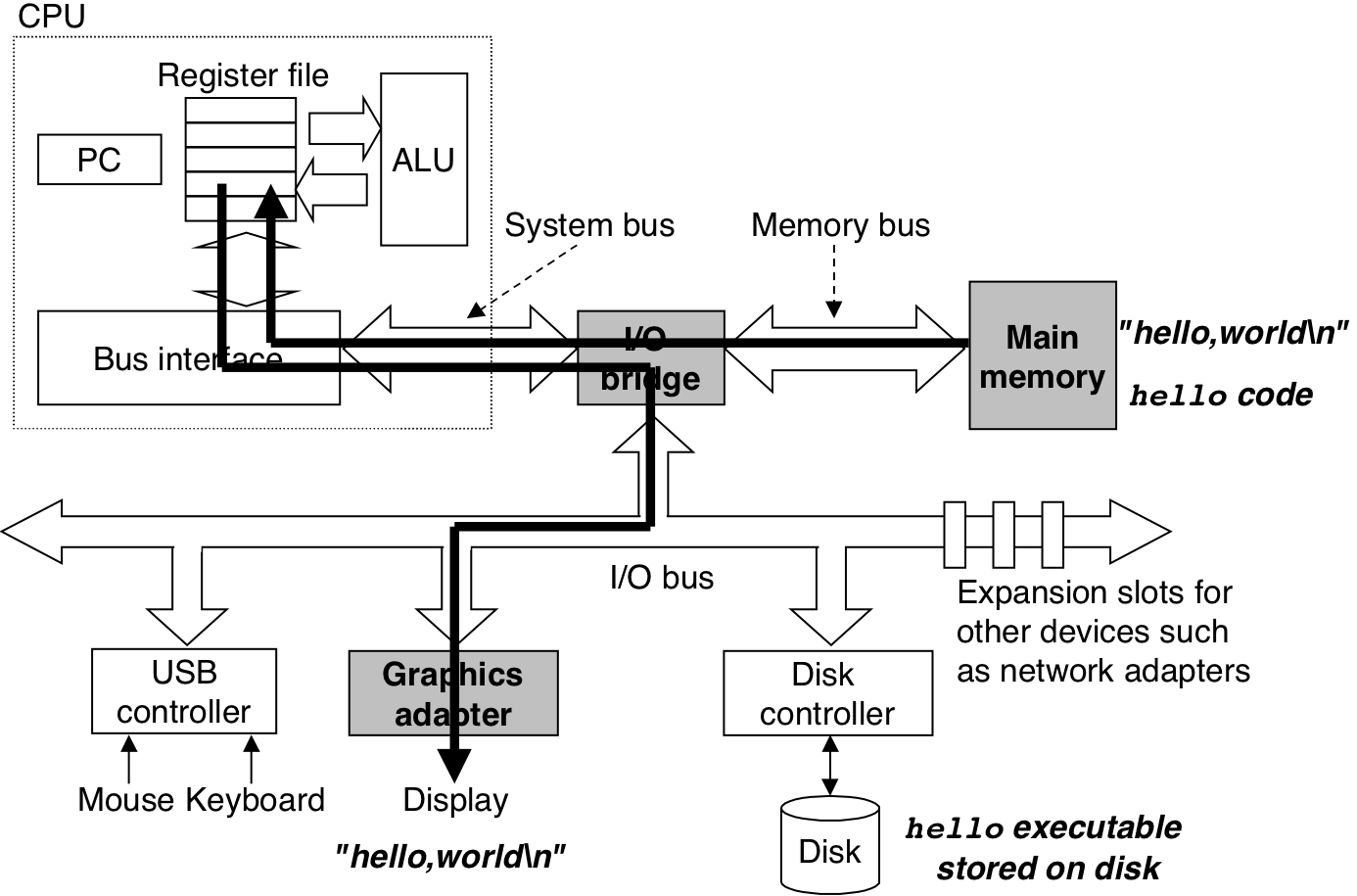
Figure 1.8: Cache memories.
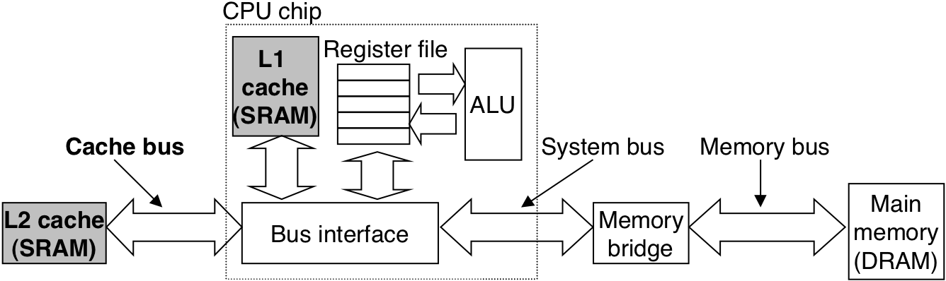
Figure 1.9: An example of a memory hierarchy.
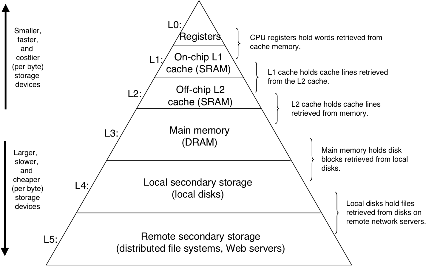
Figure 1.10: Layered view of a computer system.
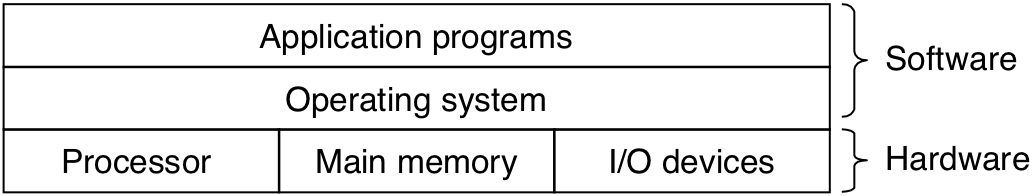
Figure 1.11: Abstractions provided by an operating system.
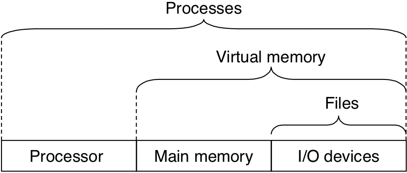
Figure 1.12: Process context switching.
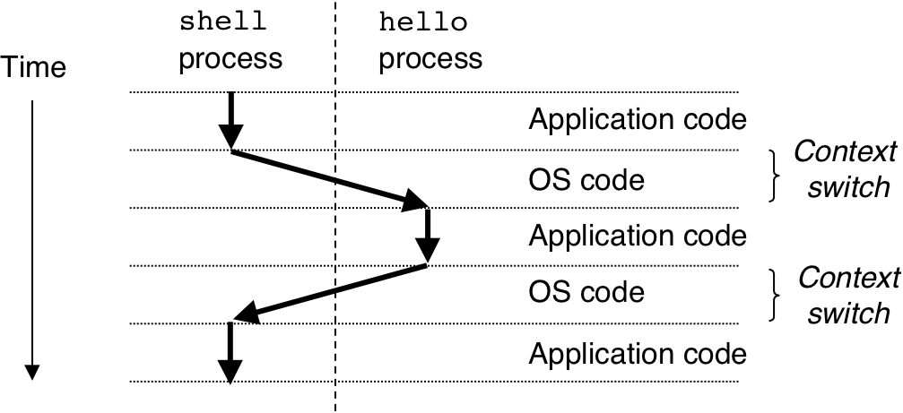
Figure 1.13: Process virtual address space.
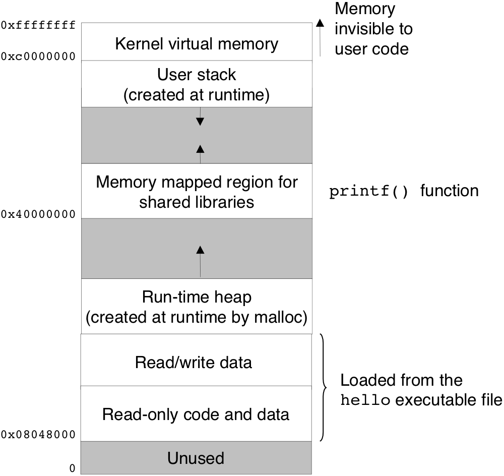
Figure 1.14: A network is another I/O device.
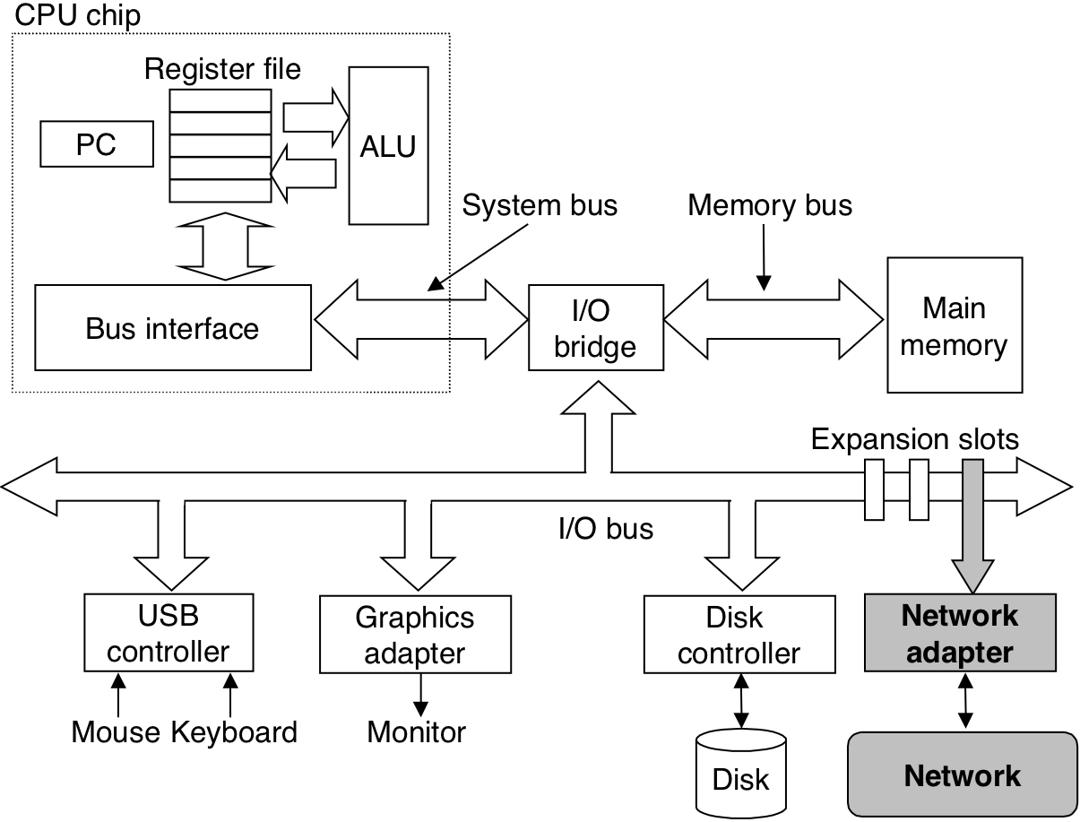
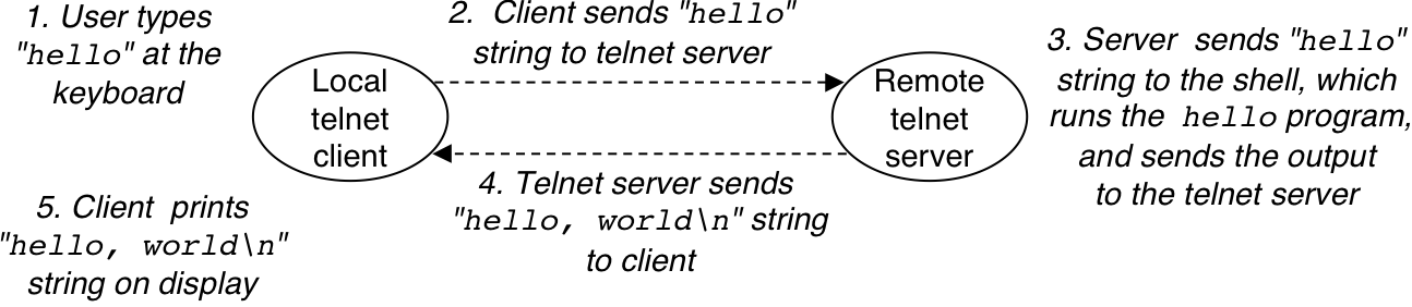
Figure 1.15: Using telnet to run hello remotely over a network.
| 2 [2/13] |
Figure 2.11: Conversion from two's complement to unsigned.
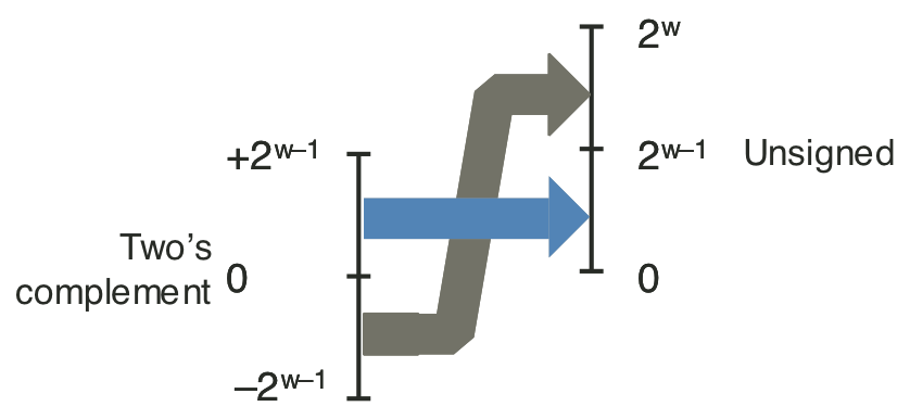
Figure 2.12: Conversion from unsigned to two's complement.
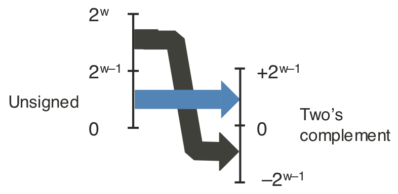
Figure 2.14: Integer addition.
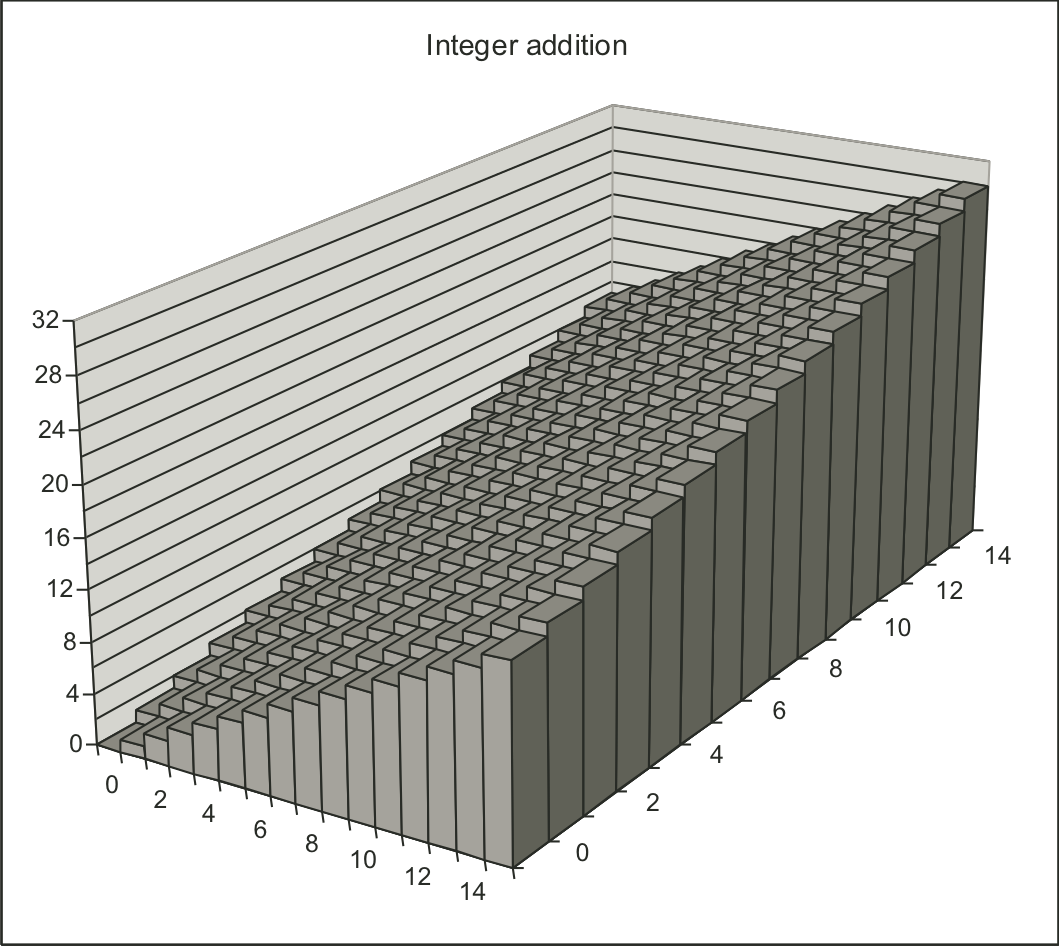
Figure 2.15: Relation between integer addition and unsigned addition.
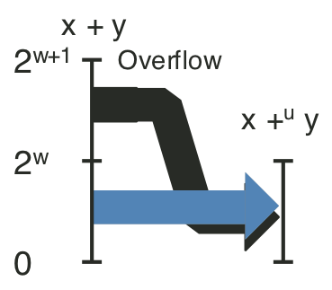
Figure 2.16: Unsigned addition.
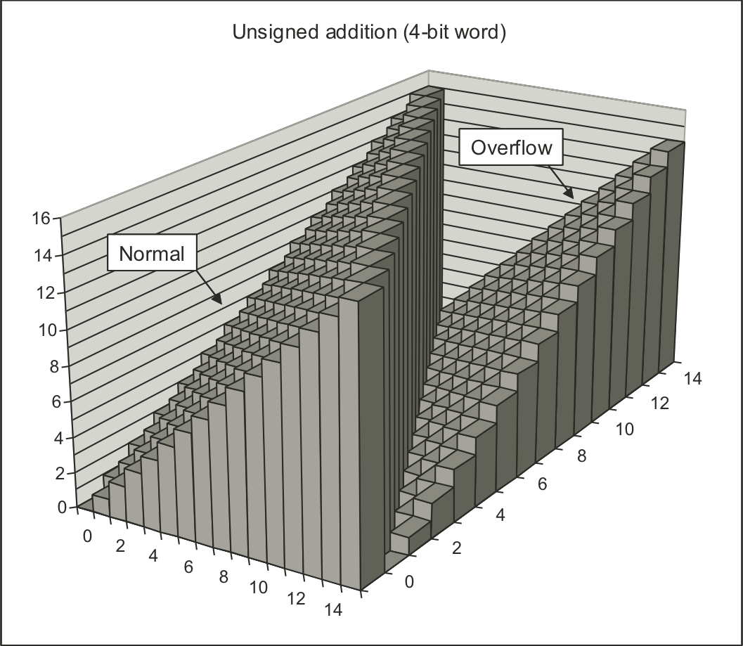
Figure 2.17: Relation between integer and two's-complement addition.
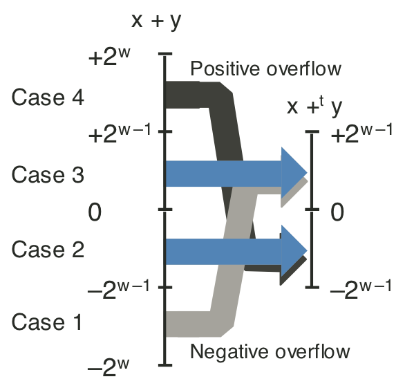
Figure 2.19: two's-complement addition.
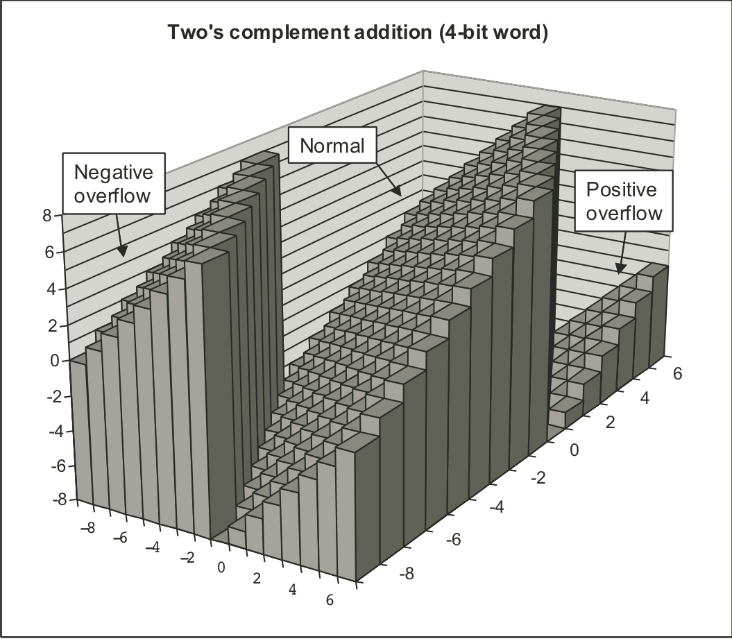
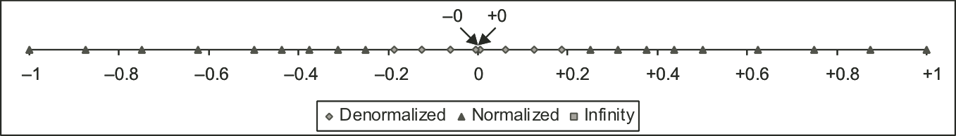
Figure 2.22: Representable values for six-bit floating-point format.
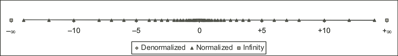
Figure 2.22: Representable values for six-bit floating-point format.
| 3 [3/13] |
Figure 3.5: Illustration of stack operation.
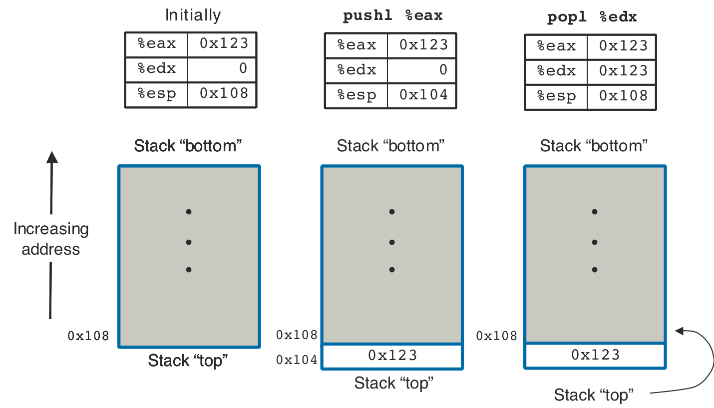
Figure 3.17: Stack frame structure.
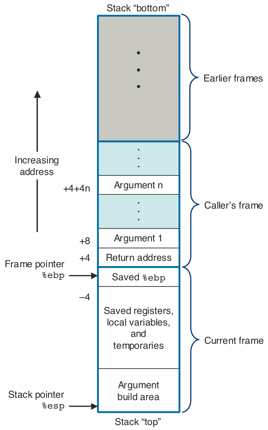
Figure 3.19: Stack frames for caller and swap_add.
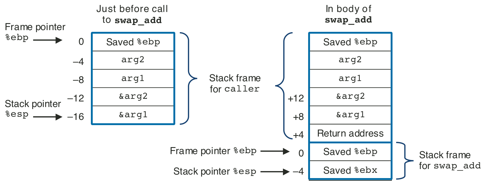
Figure 3.22: Stack frame for recursive Fibonacci function.
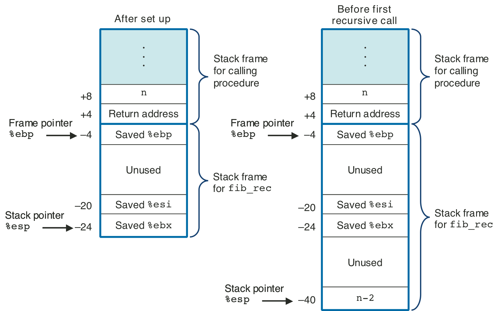
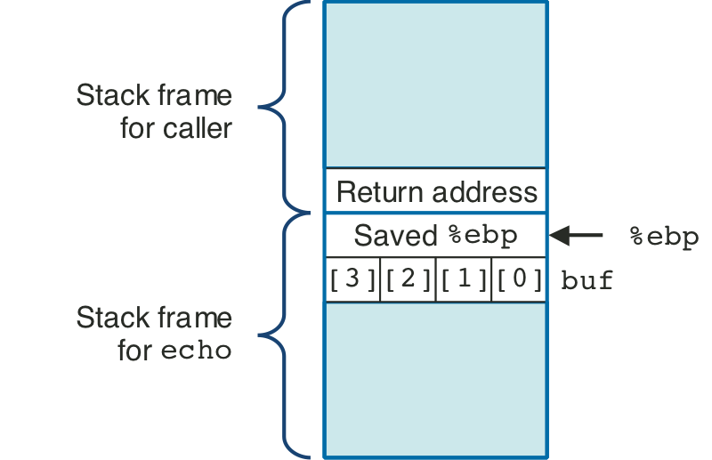
Figure 3.28: Stack organization for echo function.
| 4 [4/13] |
Figure 4.1: Y86 programmer-visible state.
Figure 4.2: Y86 instruction set.
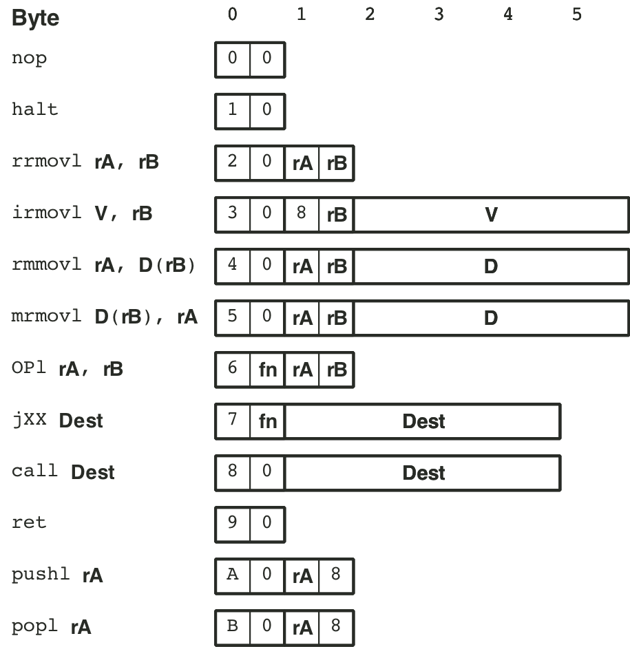
Figure 4.3: Function codes for Y86 instruction set.
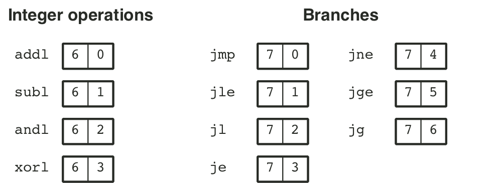
Figure 4.8: Logic gate types.
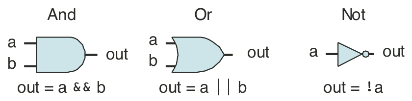
Figure 4.9: Combinational circuit to test for bit equality.
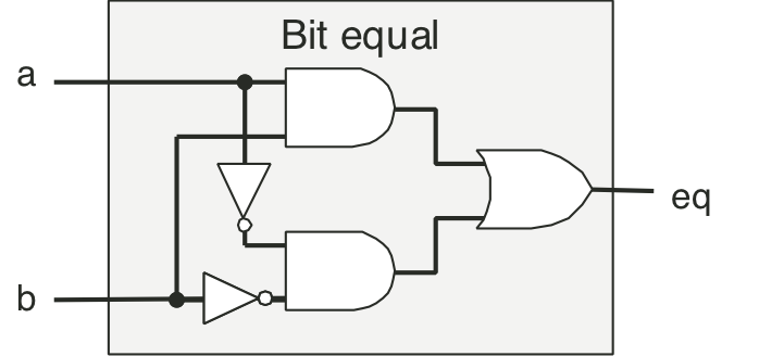
Figure 4.10: Single-bit multiplexor circuit.
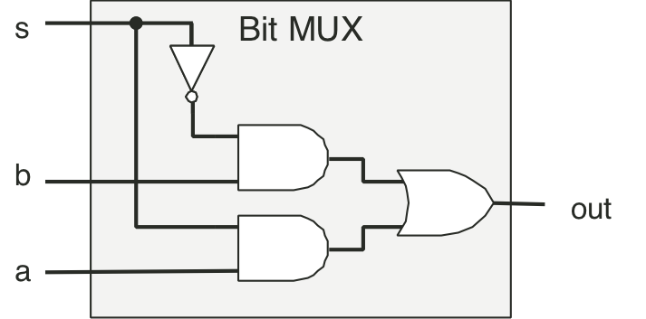
Figure 4.11: Word-level equality test circuit.
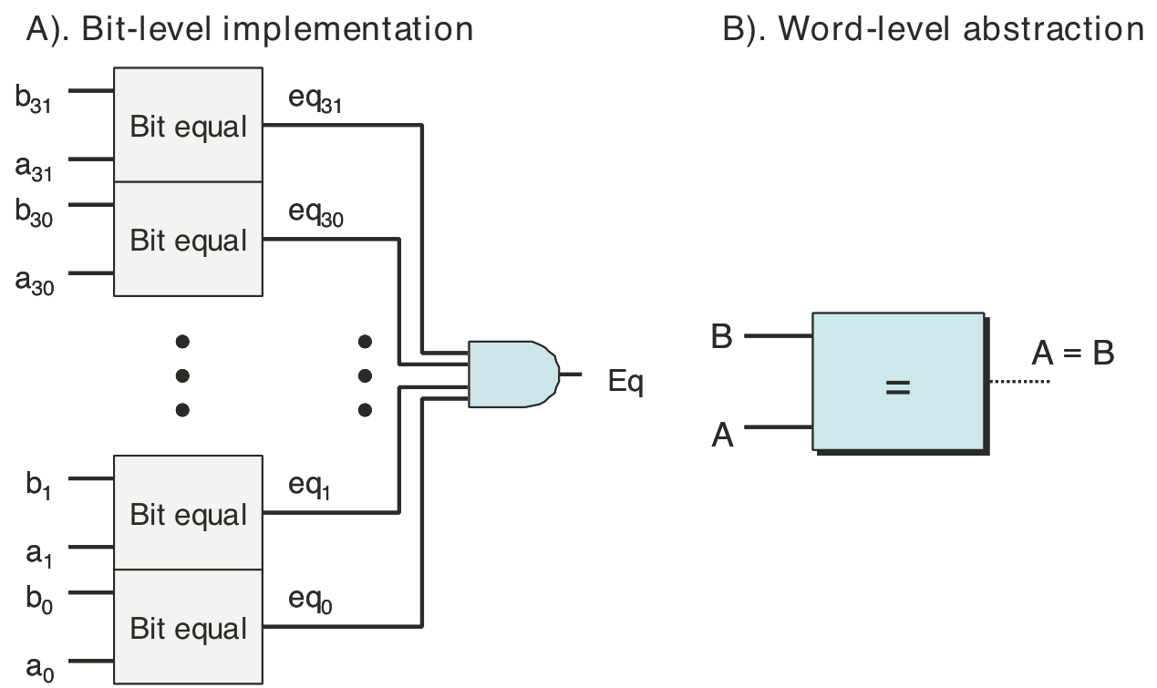
Figure 4.12: Word-level multiplexor circuit.
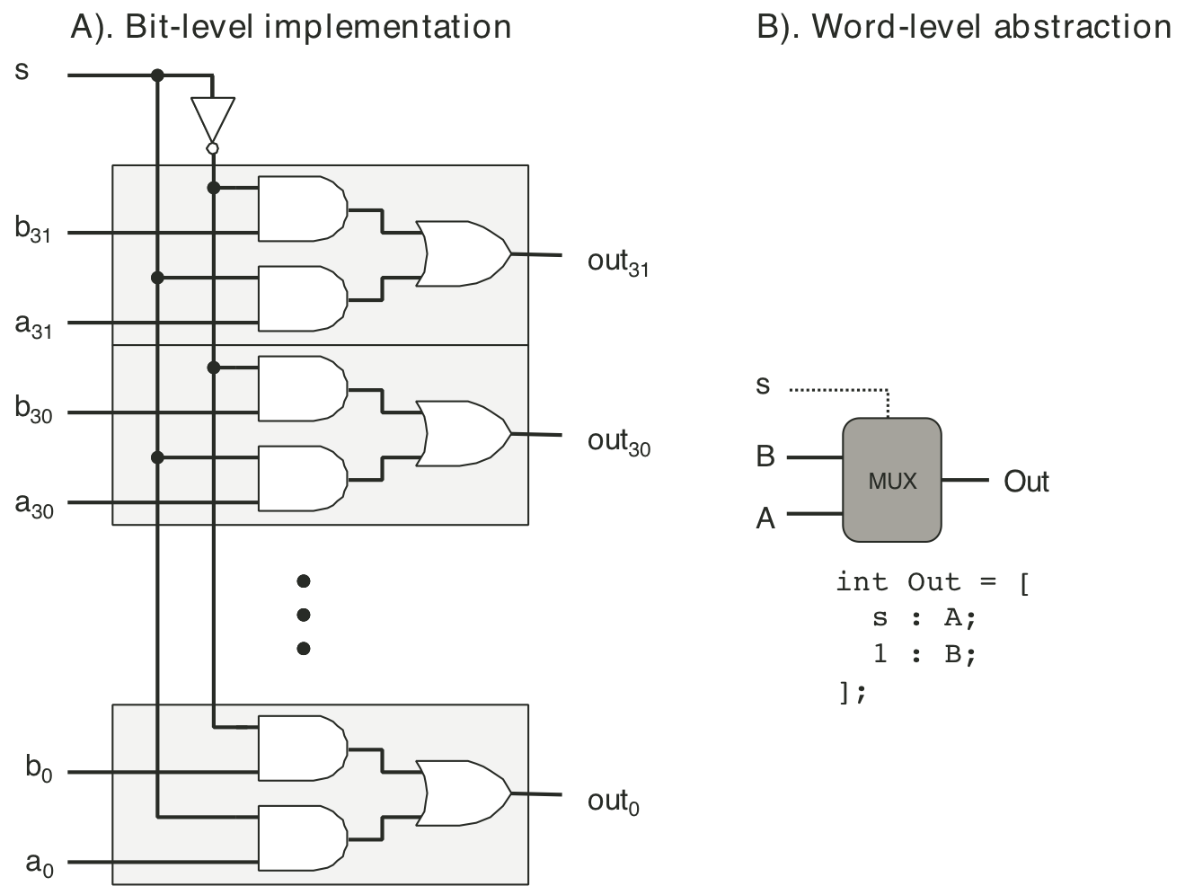
Figure 4.13: Arithmetic/logic unit (ALU).
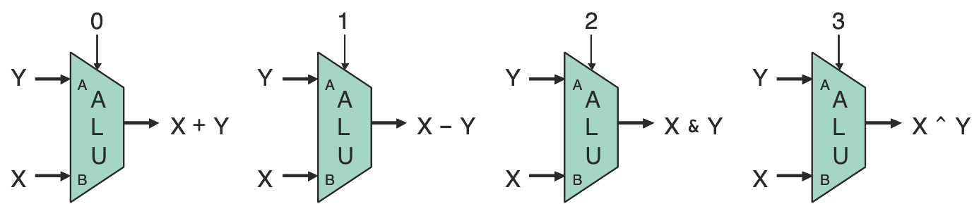
Figure 4.14: Register operation.
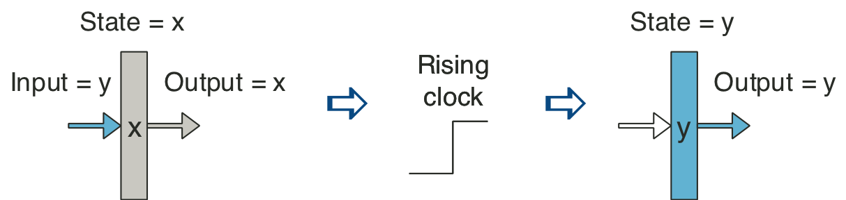
Figure 4.20: Abstract view of SEQ, a sequential implementation.
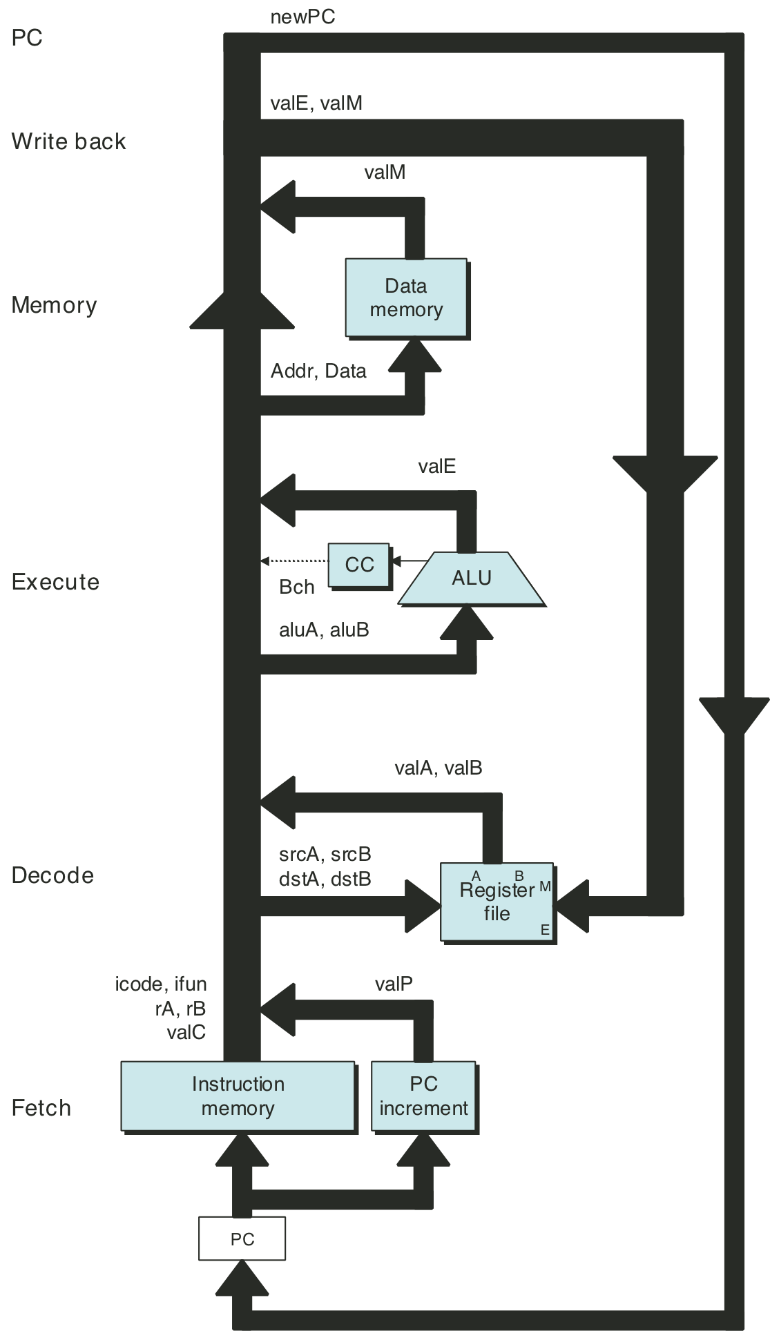
Figure 4.21: Hardware structure of SEQ, a sequential implementation.
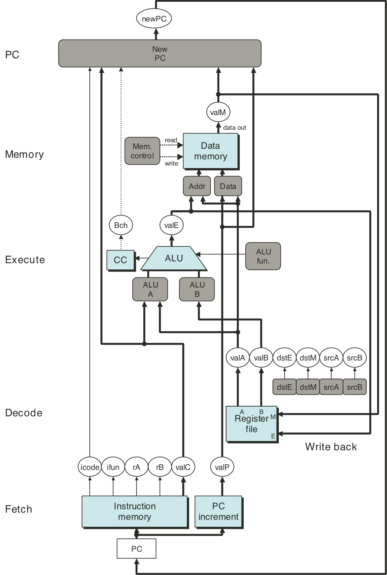
Figure 4.23: Tracing two cycles of execution by SEQ.
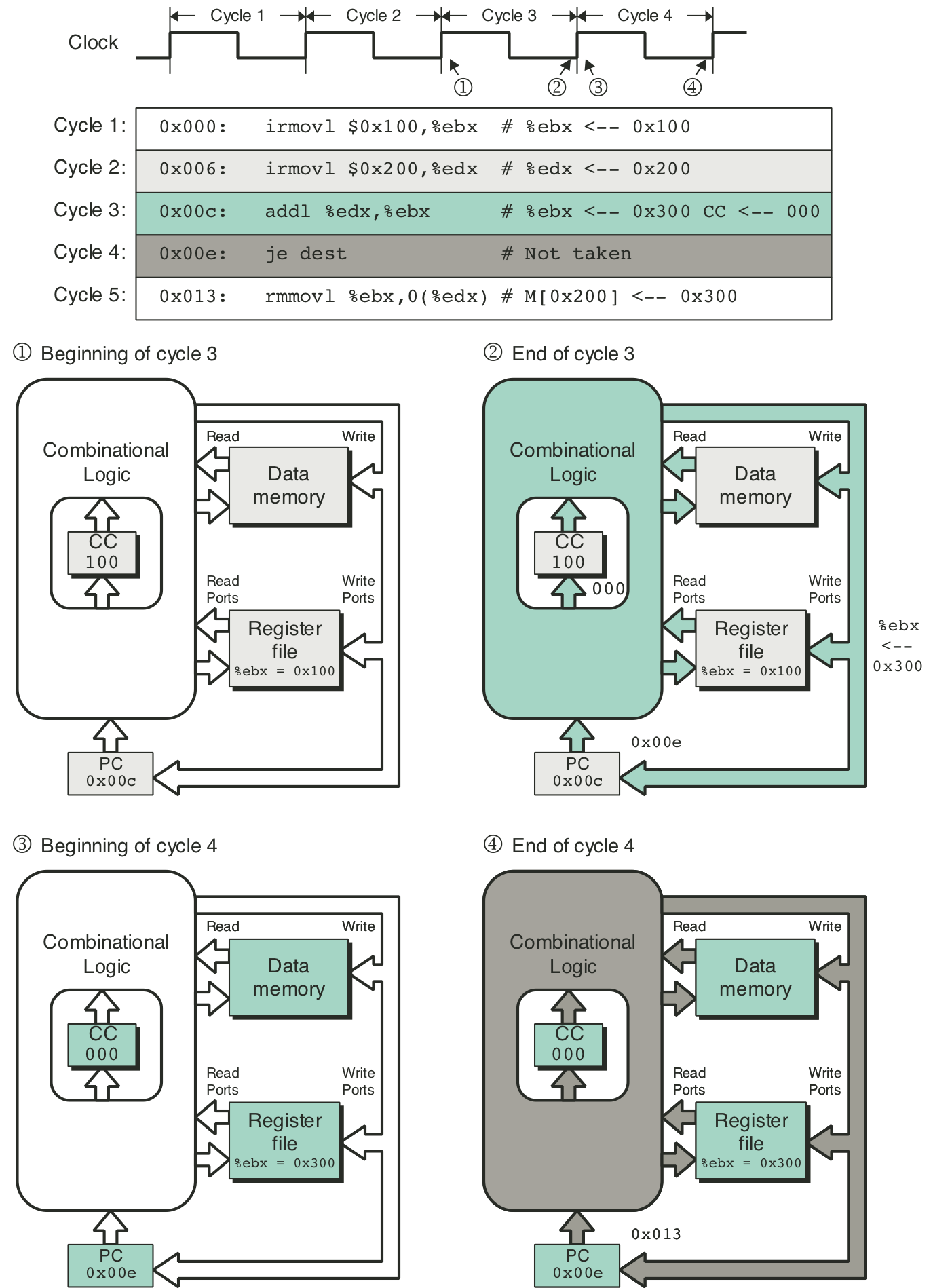
Figure 4.25: SEQ fetch stage.
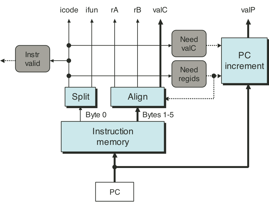
Figure 4.26: SEQ decode and write-back stage.
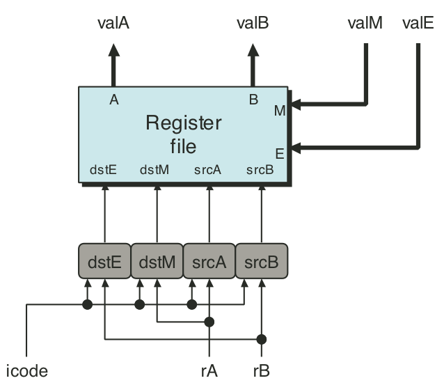
Figure 4.27: SEQ execute stage.
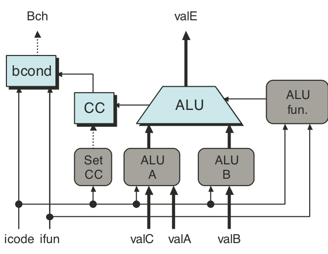
Figure 4.28: SEQ memory stage.
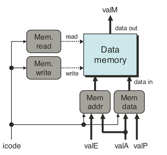
Figure 4.29: SEQ PC update stage.
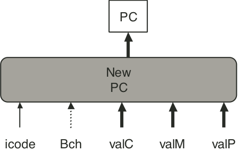
Figure 4.30: SEQ+ abstract view.
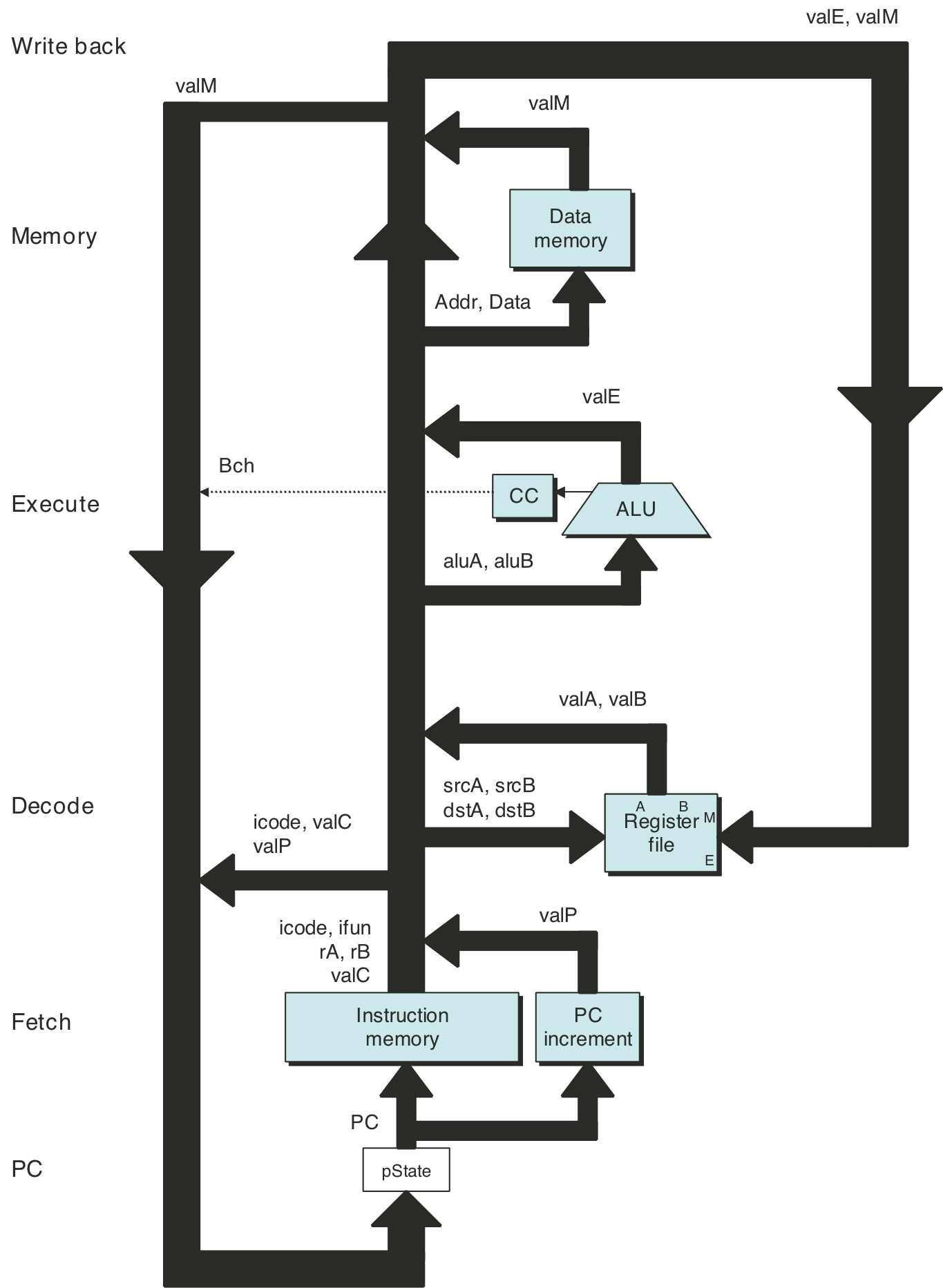
Figure 4.31: SEQ+ hardware structure.
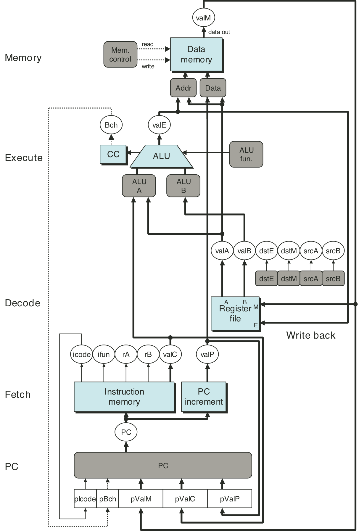
Figure 4.32: Unpipelined computation hardware.
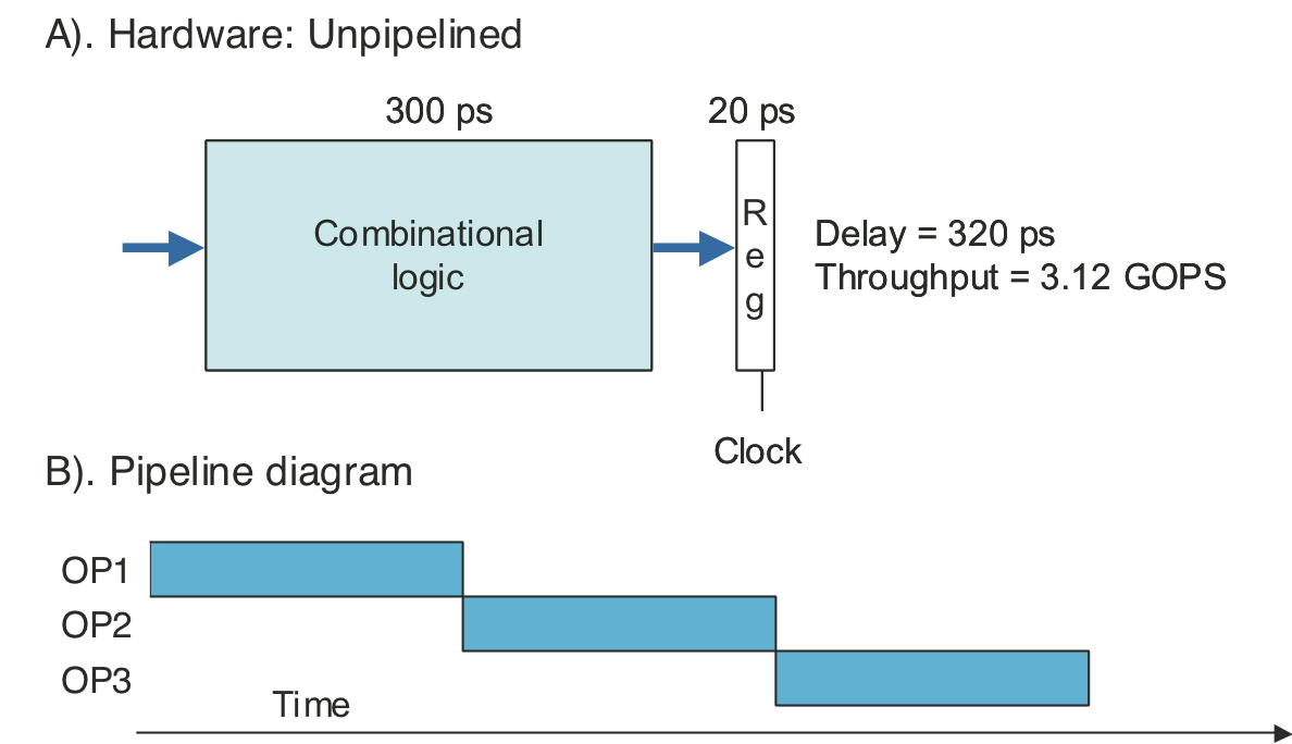
Figure 4.33: Three-stage pipelined computation hardware.
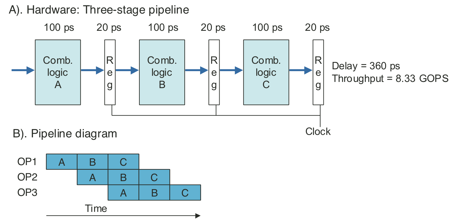
Figure 4.34: Three-stage pipeline timing.
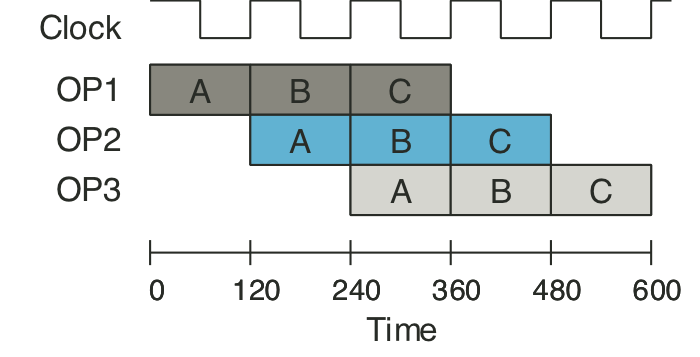
Figure 4.35: One clock cycle of pipeline operation.
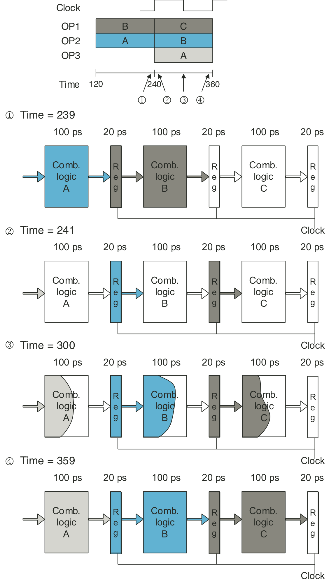
Figure 4.36: Limitations of pipelining due to nonuniform stage delays.
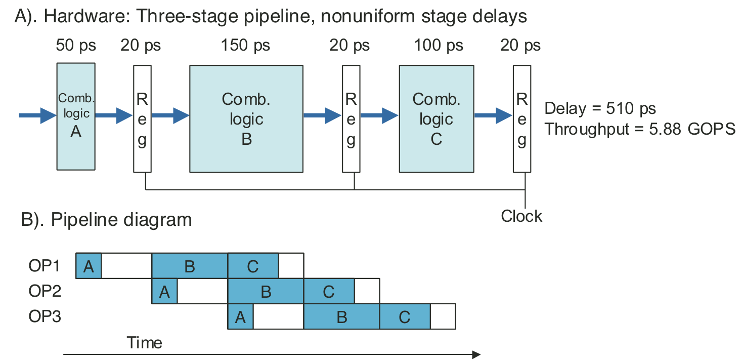
Figure 4.37: Limitations of pipelining due to overhead.
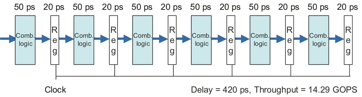
Figure 4.38: Limitations of pipelining due to logical dependencies.
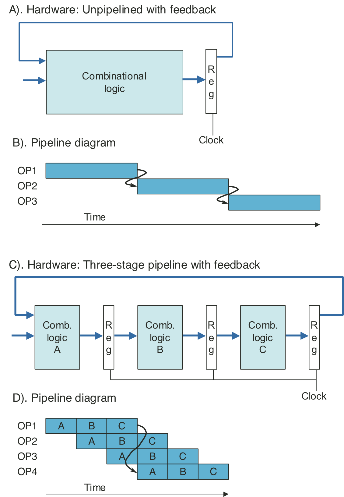
Figure 4.39: Abstract view of PIPE-, an initial pipelined implementation.
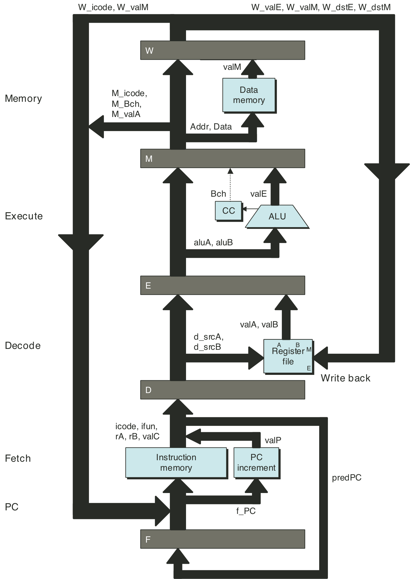
Figure 4.40: Example of instruction flow through pipeline.
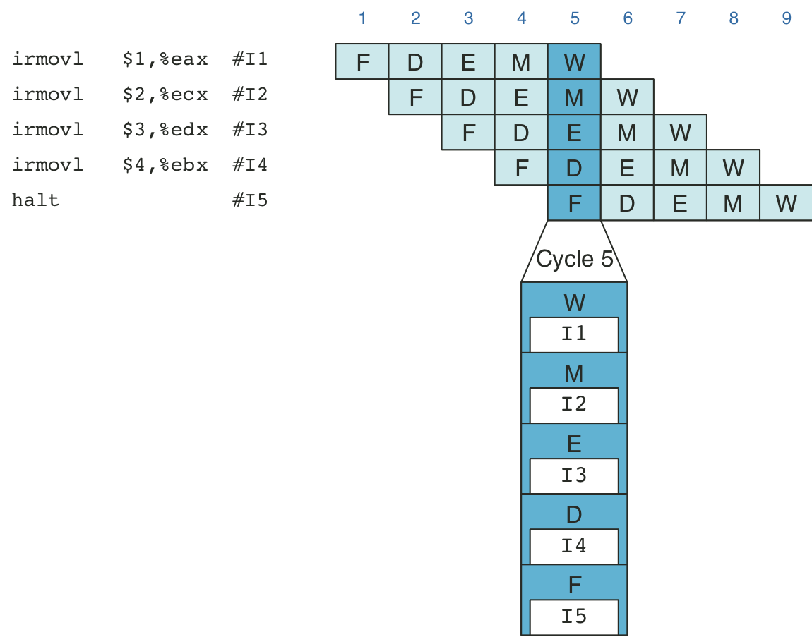
Figure 4.41: Hardware structure of PIPE-, an initial pipelined implementation.
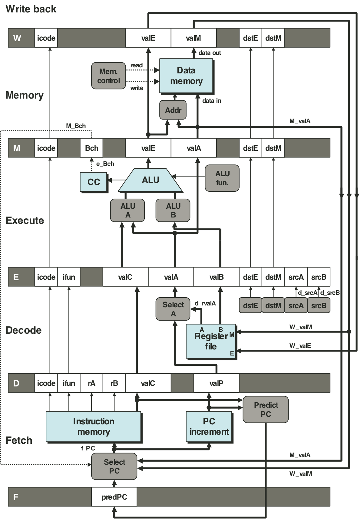
Figure 4.42: Pipelined execution of prog1 without special pipeline control.
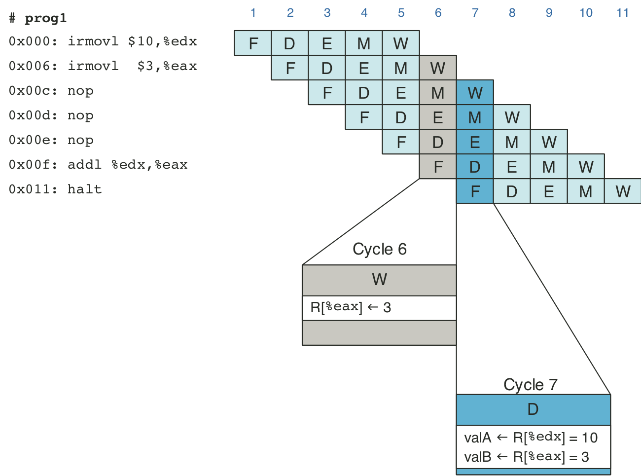
Figure 4.43: Pipelined execution of prog2 without special pipeline control.
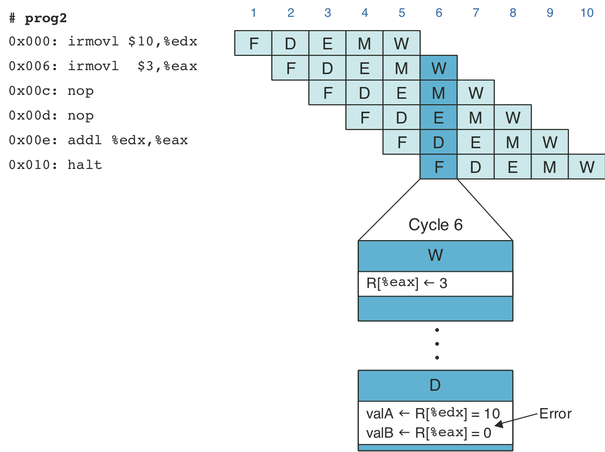
Figure 4.44: Pipelined execution of prog3 without special pipeline control.
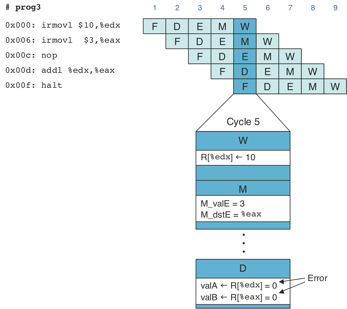
Figure 4.45: Pipelined execution of prog4 without special pipeline control.
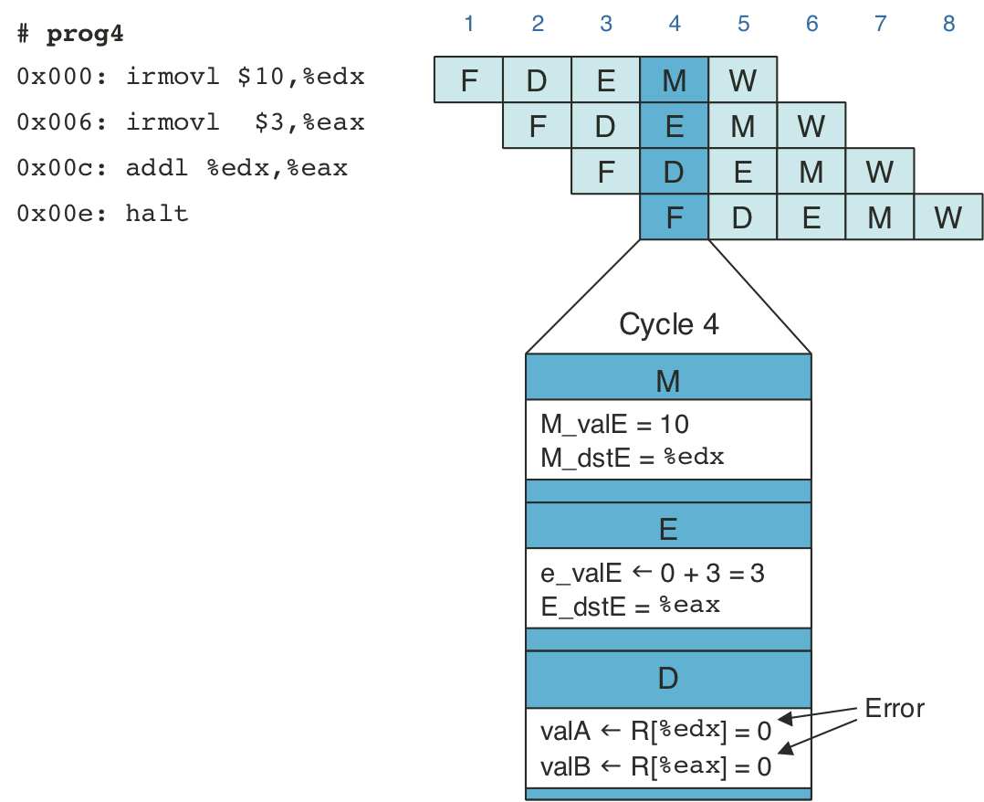
Figure 4.46: Pipelined execution of prog2 using stalls.
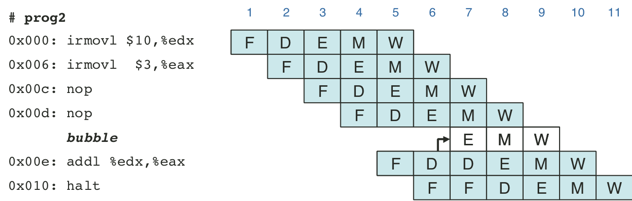
Figure 4.47: Pipelined execution of prog3 using stalls.
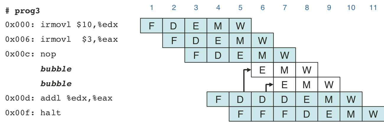
Figure 4.48: Pipelined execution of prog4 using stalls.
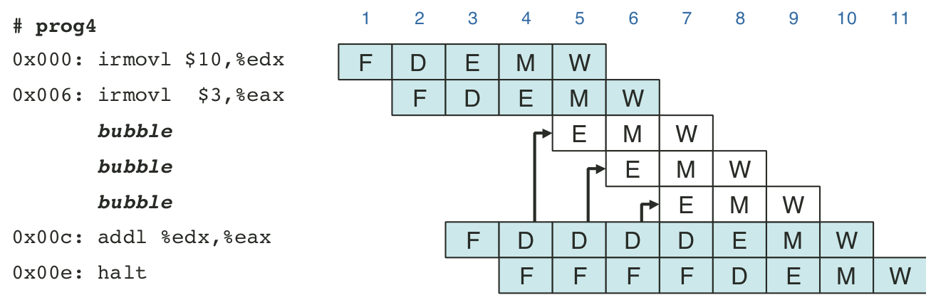
Figure 4.49: Pipelined execution of prog2 using forwarding.
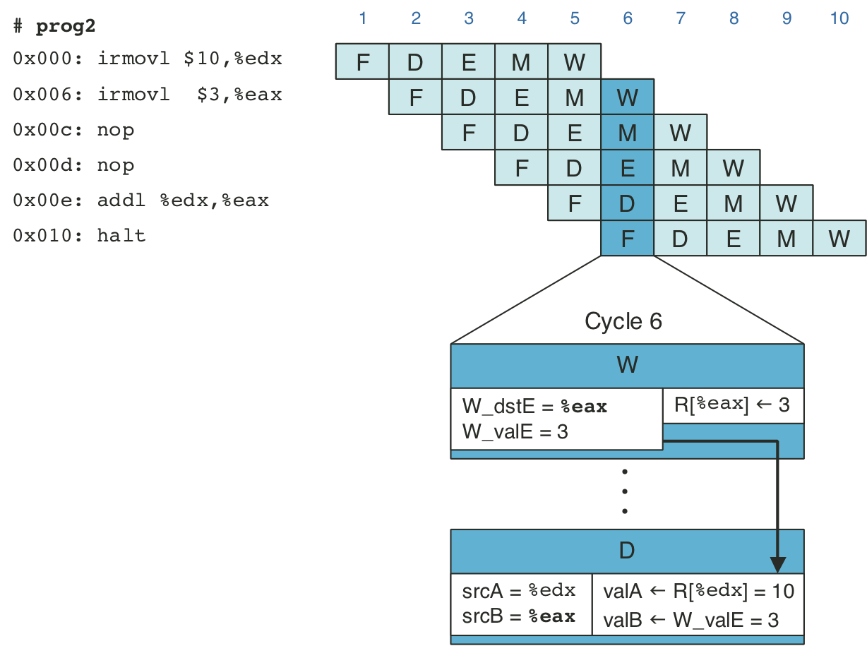
Figure 4.50: Pipelined execution of prog3 using forwarding.
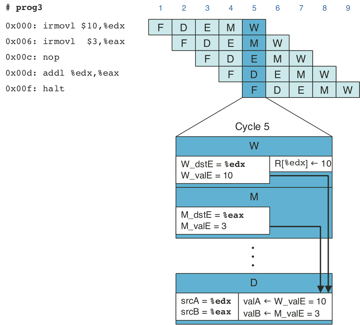
Figure 4.51: Pipelined execution of prog4 using forwarding.
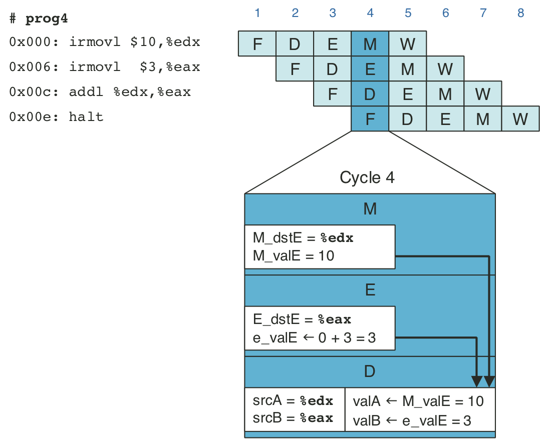
Figure 4.52: Abstract view of PIPE, our final pipelined implementation.
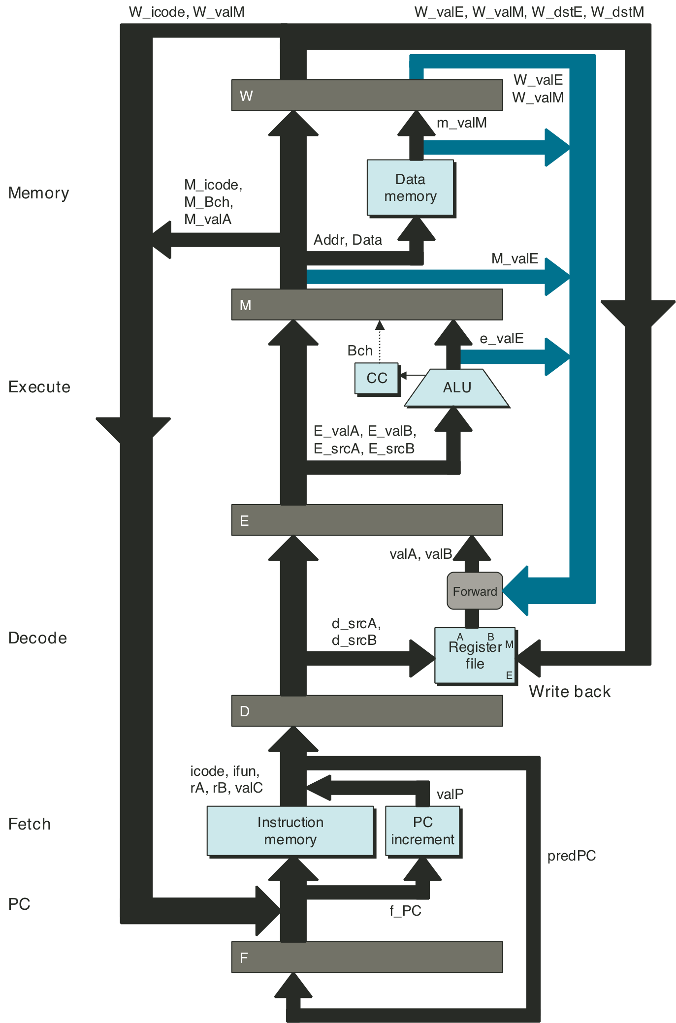
Figure 4.53: Hardware structure of PIPE, our final pipelined implementation.
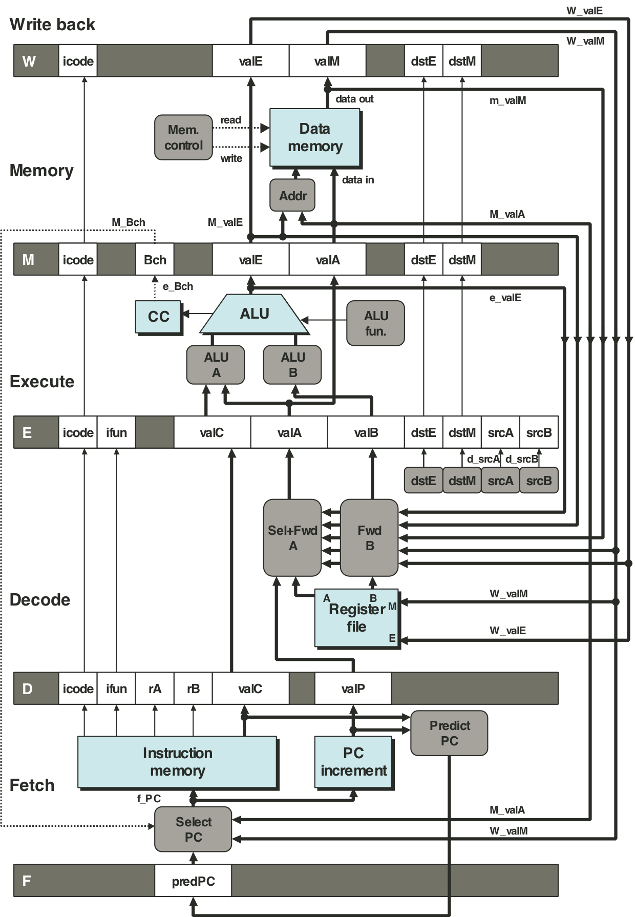
Figure 4.54: Example of load/use data hazard.
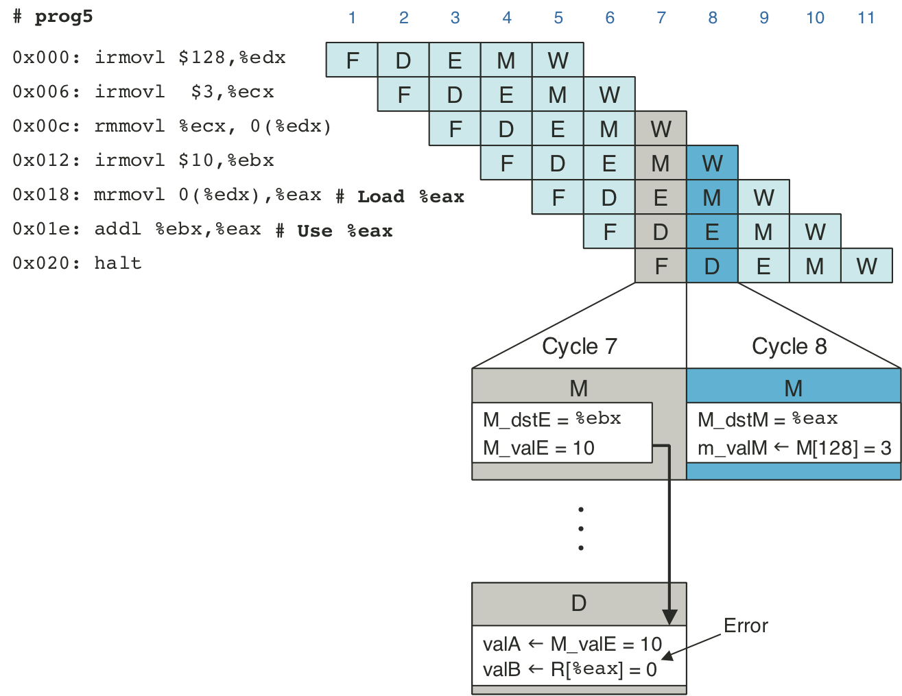
Figure 4.55: Handling a load/use hazard by stalling.
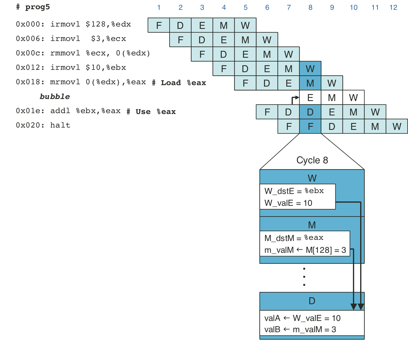
Figure 4.56: PIPE PC selection and fetch logic.
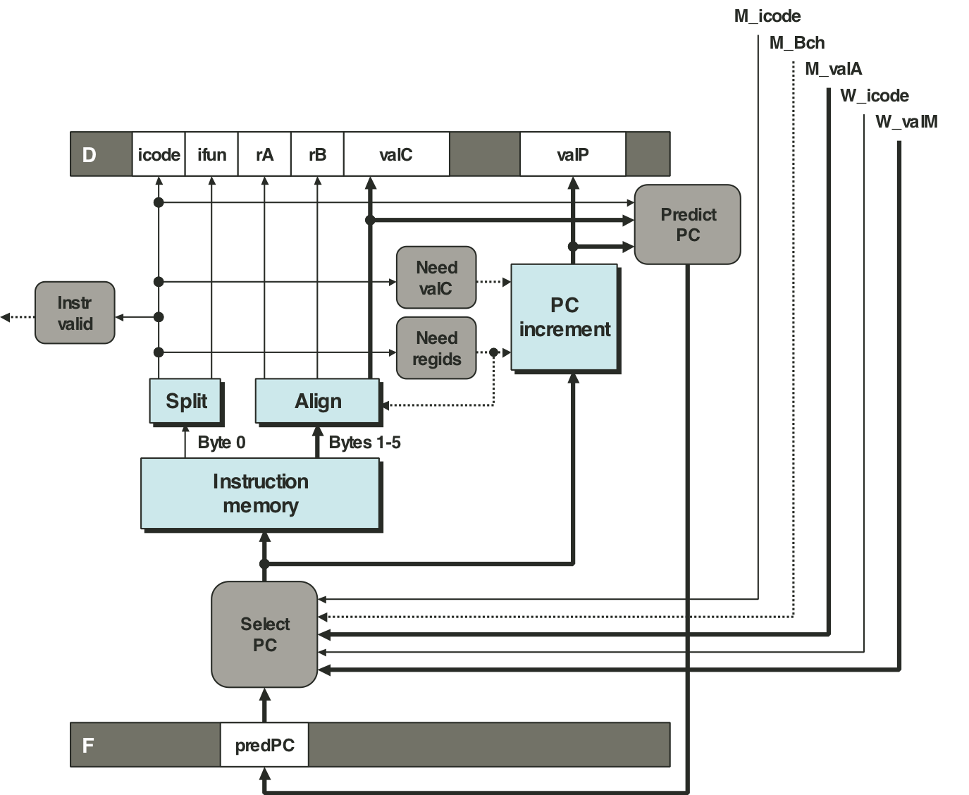
Figure 4.57: PIPE decode and write-back stage logic.
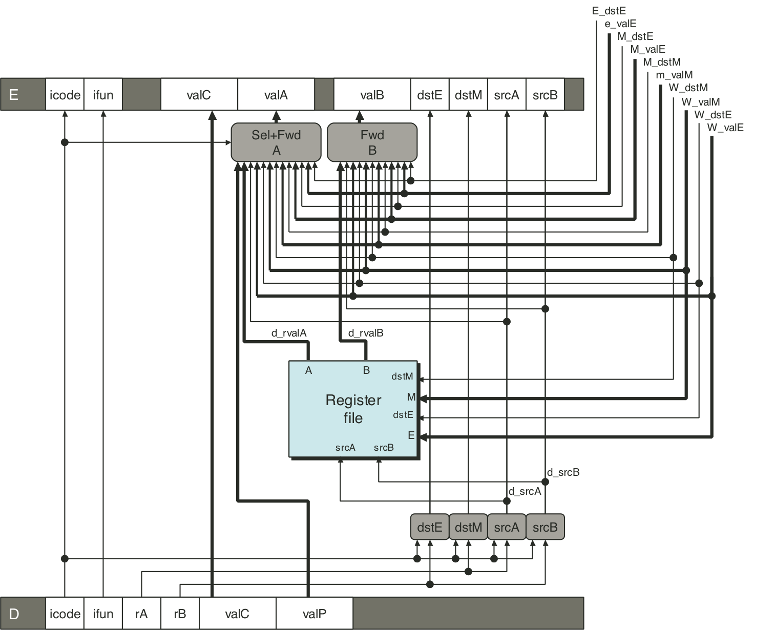
Figure 4.58: Demonstration of forwarding priority.
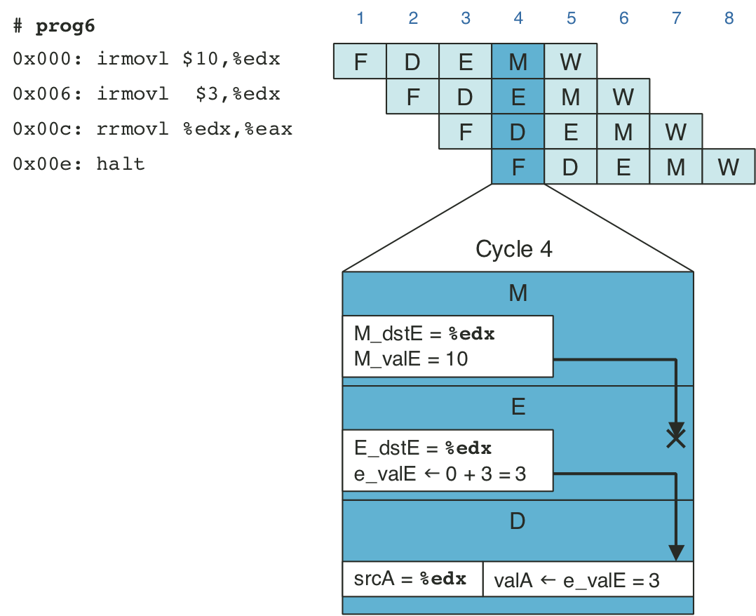
Figure 4.59: PIPE execute stage logic.
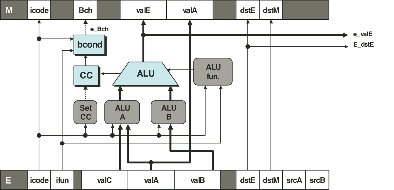
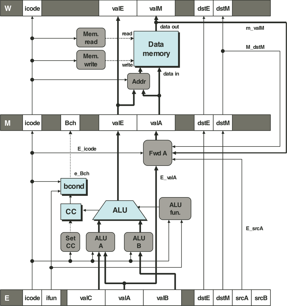
Figure 4.60: PIPE memory stage logic.
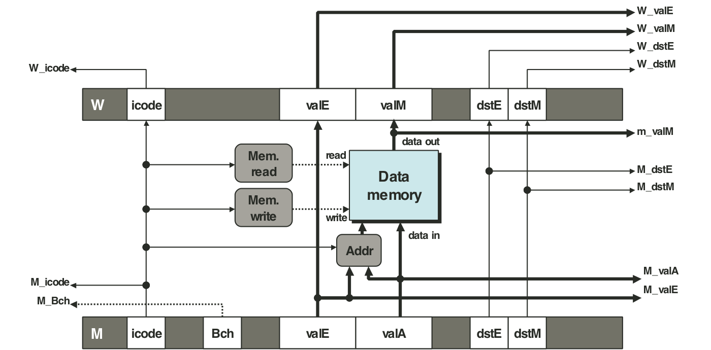
Figure 4.61: Simplified view of ret instruction processing.
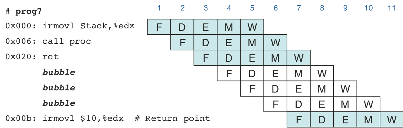
Figure 4.62: Actual processing of the ret instruction.
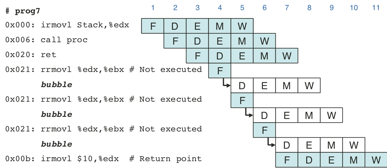
Figure 4.63: Processing mispredicted branch instructions.
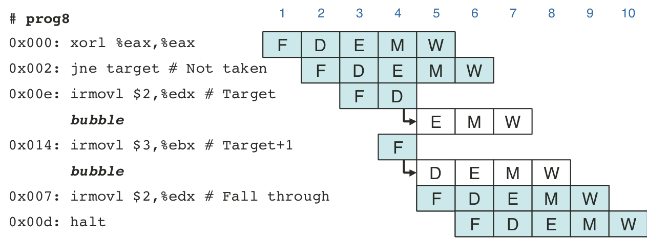
Figure 4.65: Additional pipeline register operations.
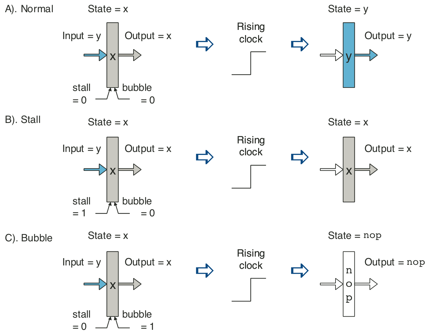
Figure 4.67: Pipeline states for special control conditions.
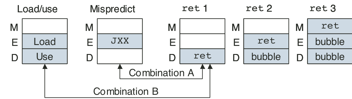
Figure 4.68: PIPE pipeline control logic.
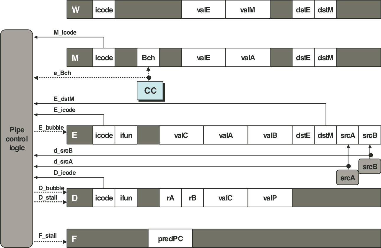
Figure 4.69: Execute and memory stages capable of load forwarding.
| 5 [5/13] |
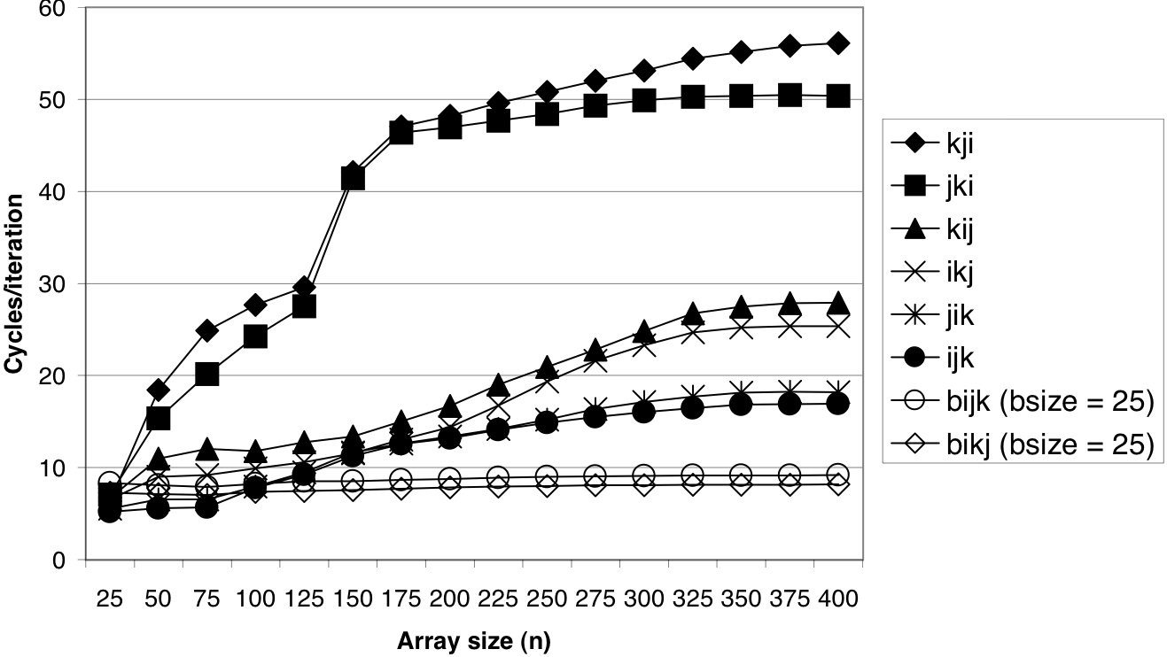
Figure 5.2: Performance of vector sum functions.
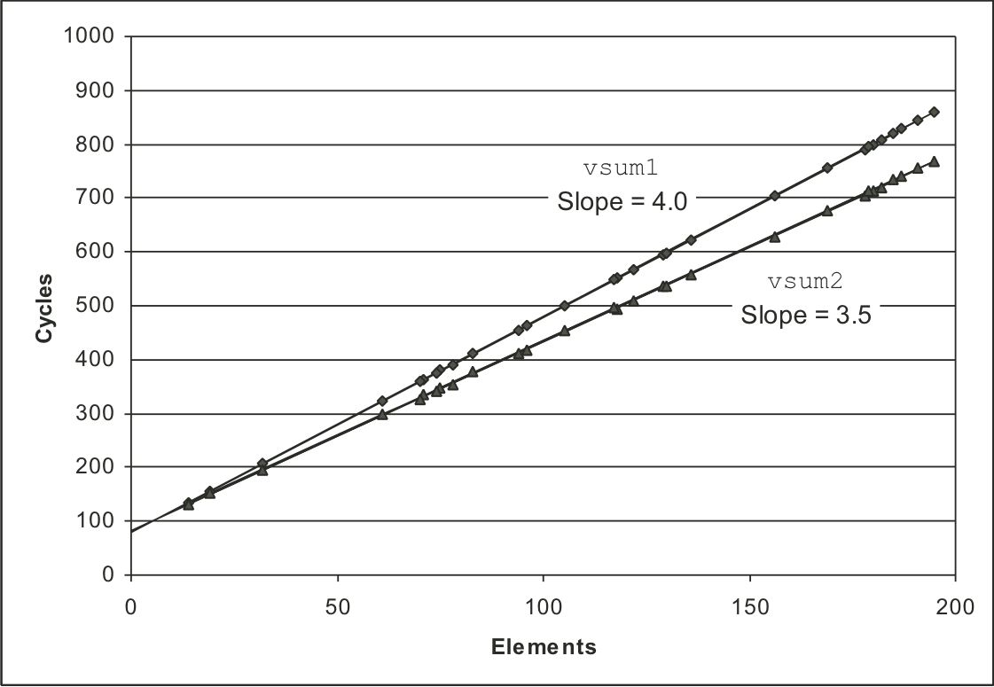
Figure 5.3: Vector abstract data type.

Figure 5.8: Comparative performance of lower-case conversion routines.
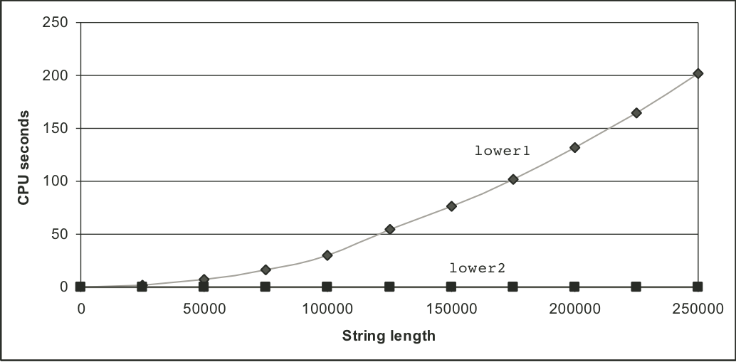
Figure 5.11: Block diagram of a modern processor.
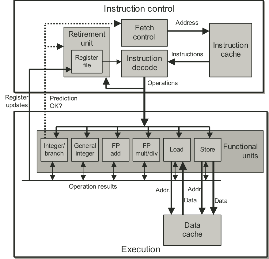
Figure 5.13: Operations for first iteration of inner loop of combine4 for integer multiplication.
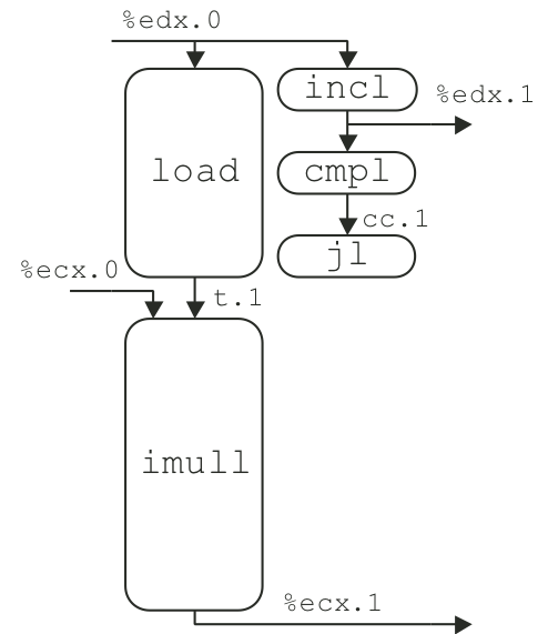
Figure 5.14: Operations for first iteration of inner loop of combine4 for integer addition.
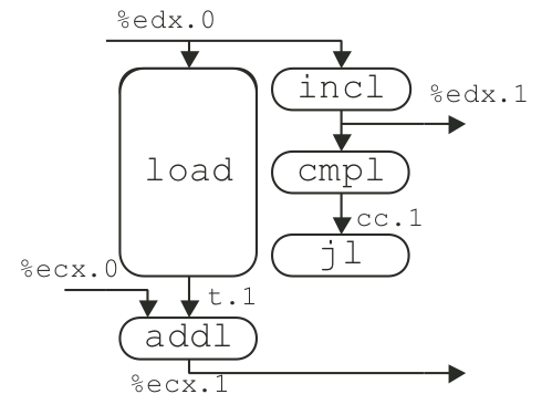
Figure 5.15: Scheduling of operations for integer multiplication with unlimited number of execution units.
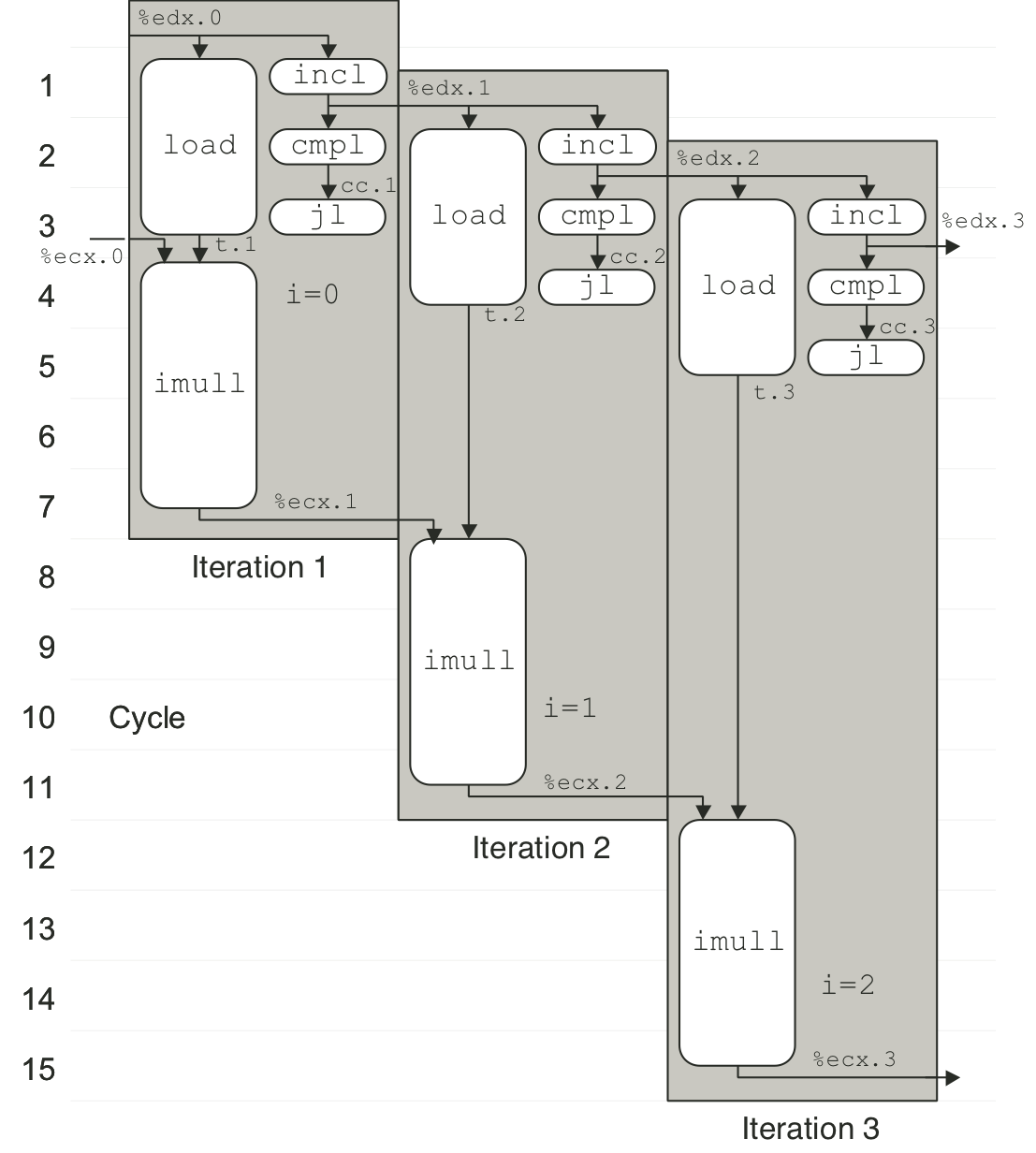
Figure 5.16: Scheduling of operations for integer addition with unbounded resource constraints.
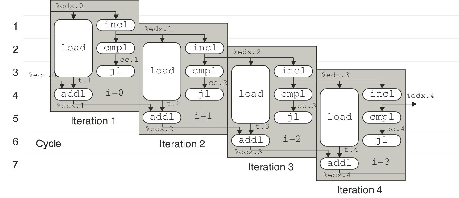
Figure 5.17: Scheduling of operations for integer multiplication with actual resource constraints.
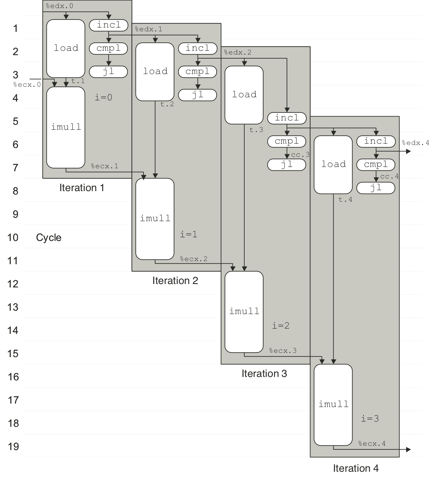
Figure 5.18: Scheduling of operations for integer addition with actual resource constraints.
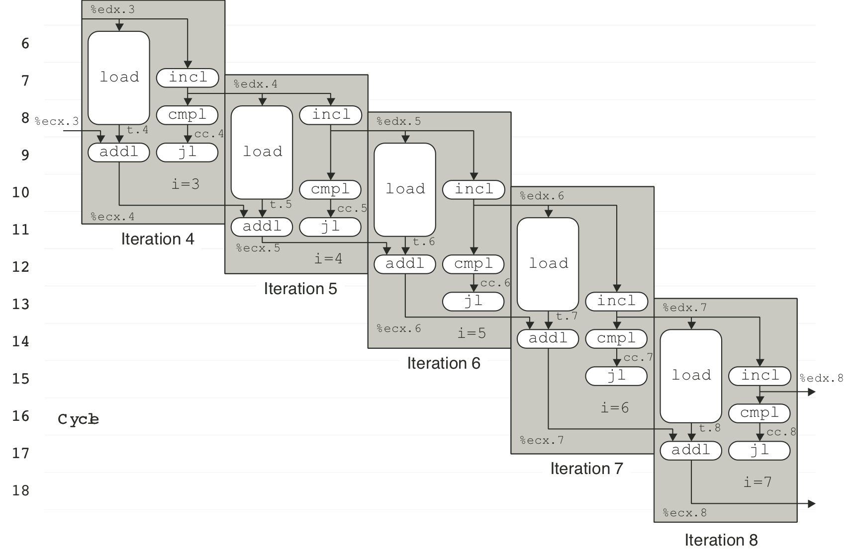
Figure 5.20: Operations for first iteration of inner loop of three-way unrolled integer addition.
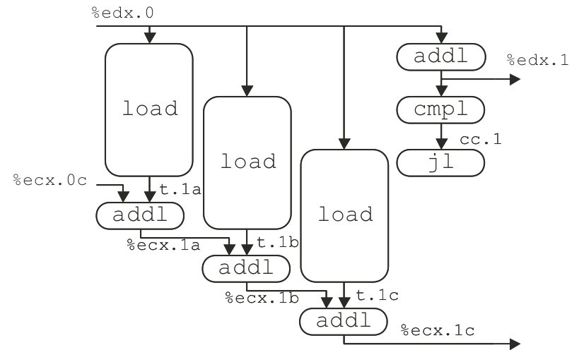
Figure 5.21: Scheduling of operations for three-way unrolled integer sum with bounded resource constraints.
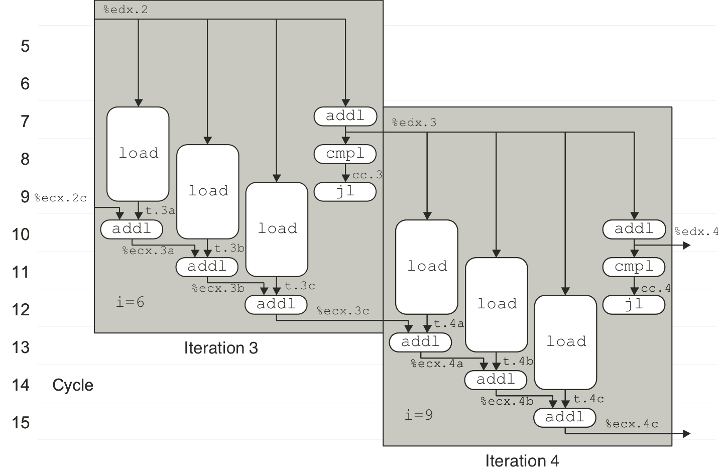
Figure 5.25: Operations for first iteration of inner loop of two-way unrolled, two-way parallel integer multiplication.
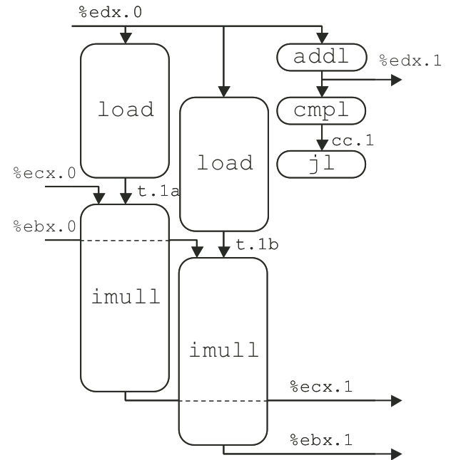
Figure 5.26: Scheduling of operations for two-way unrolled, two-way parallel integer multiplication with unlimited resources.
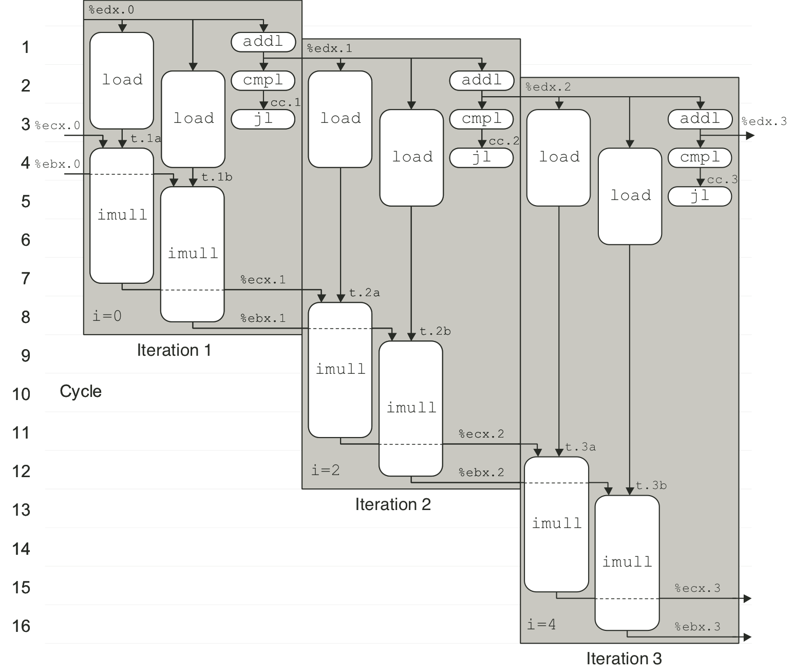
Figure 5.31: Scheduling of operations for list length function.
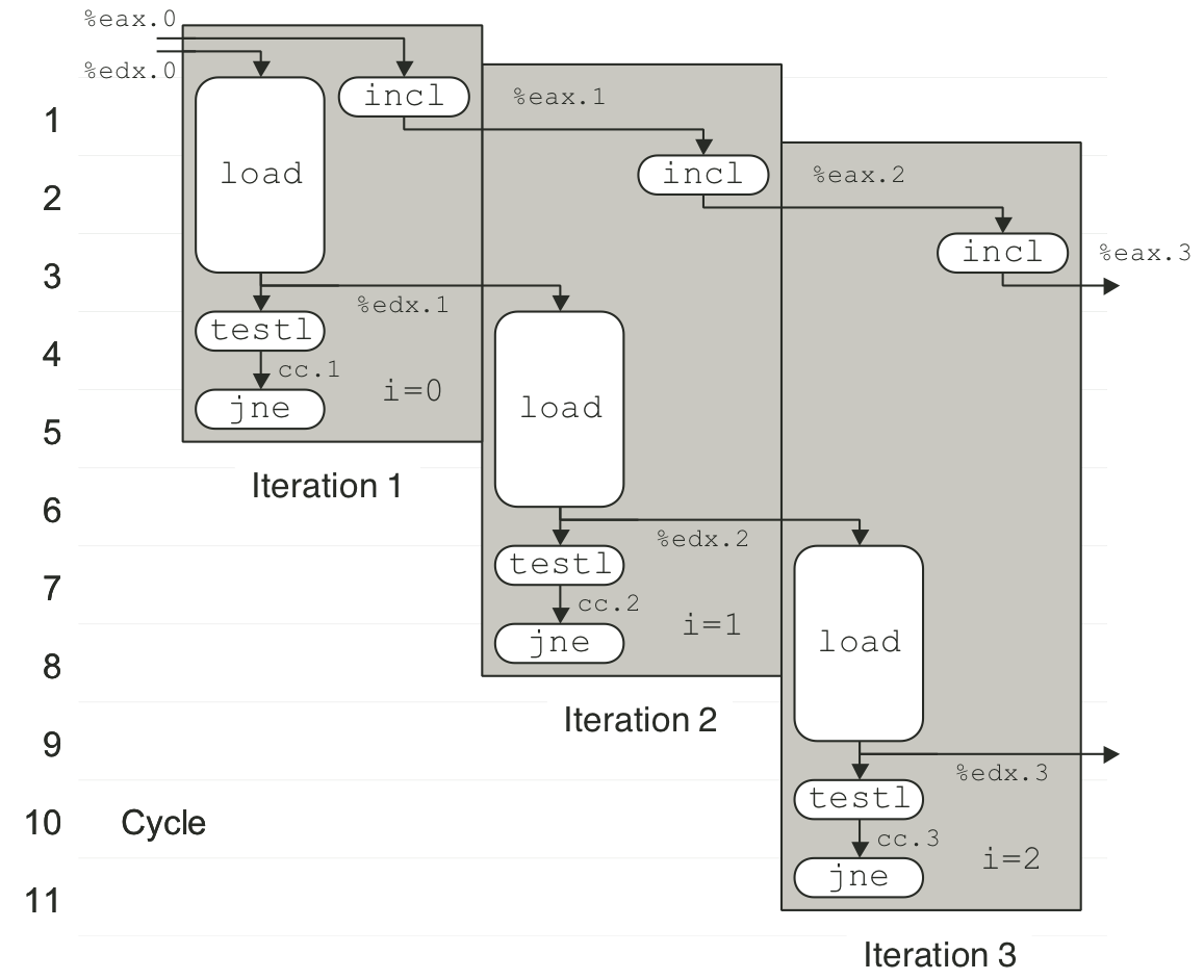
Figure 5.33: Code to write and read memory locations, along with illustrative executions.
Figure 5.34: Detail of load and store units.
Figure 5.35: Timing of write_read for example A.
Figure 5.36: Timing of write_read for example B.
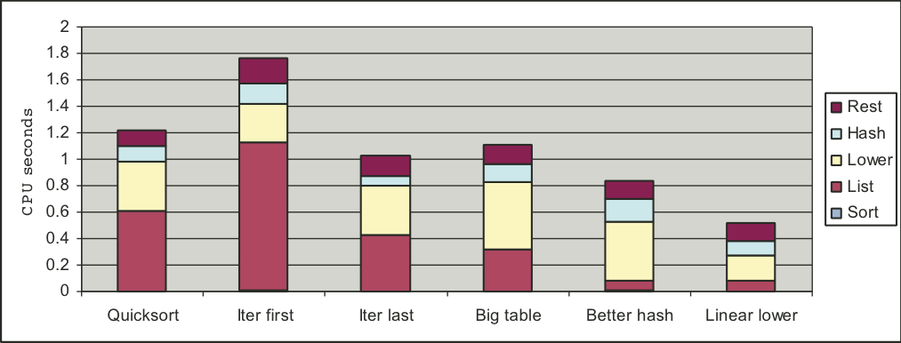
Figure 5.37: Profile results for different version of word frequency counting program.
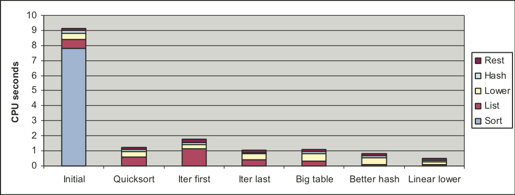
Figure 5.37: Profile results for different version of word frequency counting program.
| 6 [6/13] |
Figure 6.1: Inverted pendulum.
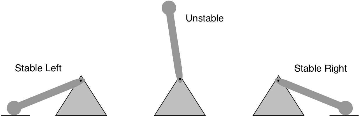
Figure 6.3: High level view of a 128-bit 16 x 8 DRAM chip.
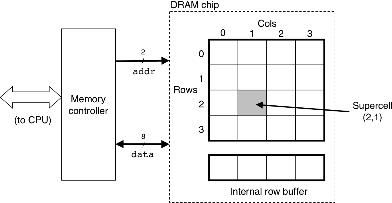
Figure 6.4: Reading the contents of a DRAM supercell.
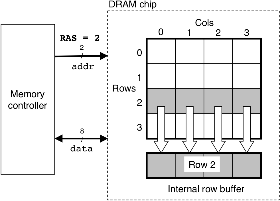
Figure 6.4: Reading the contents of a DRAM supercell.
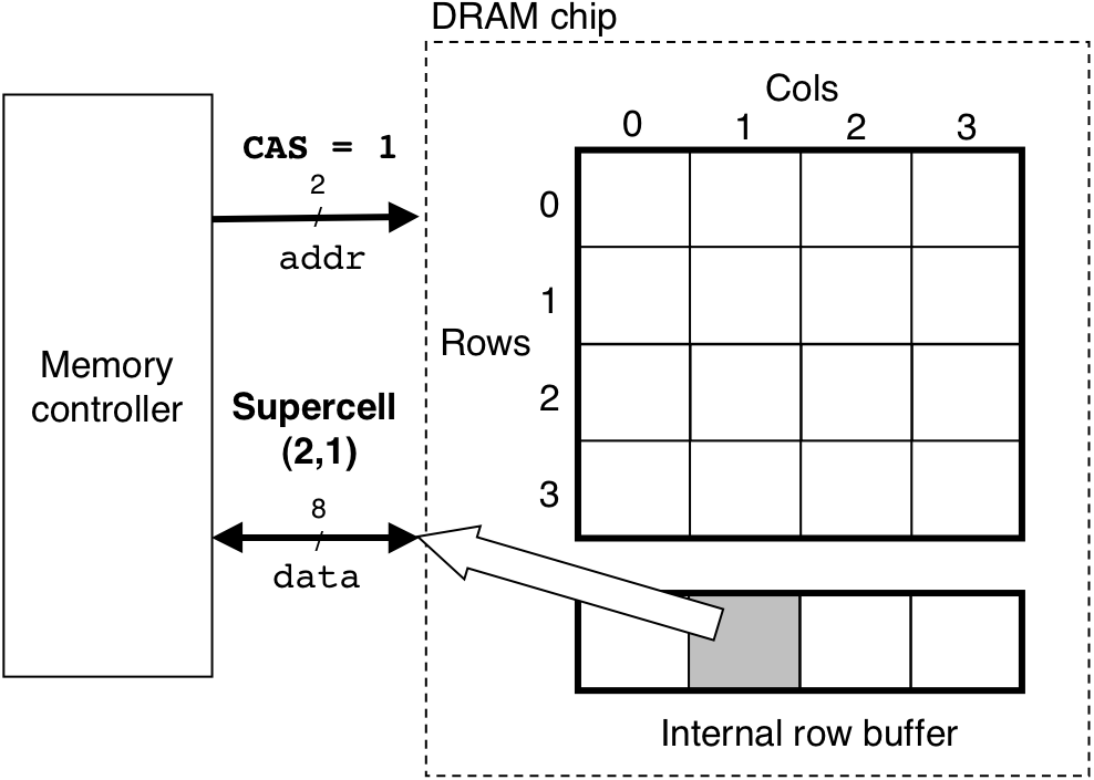
Figure 6.5: Reading the contents of a memory module.
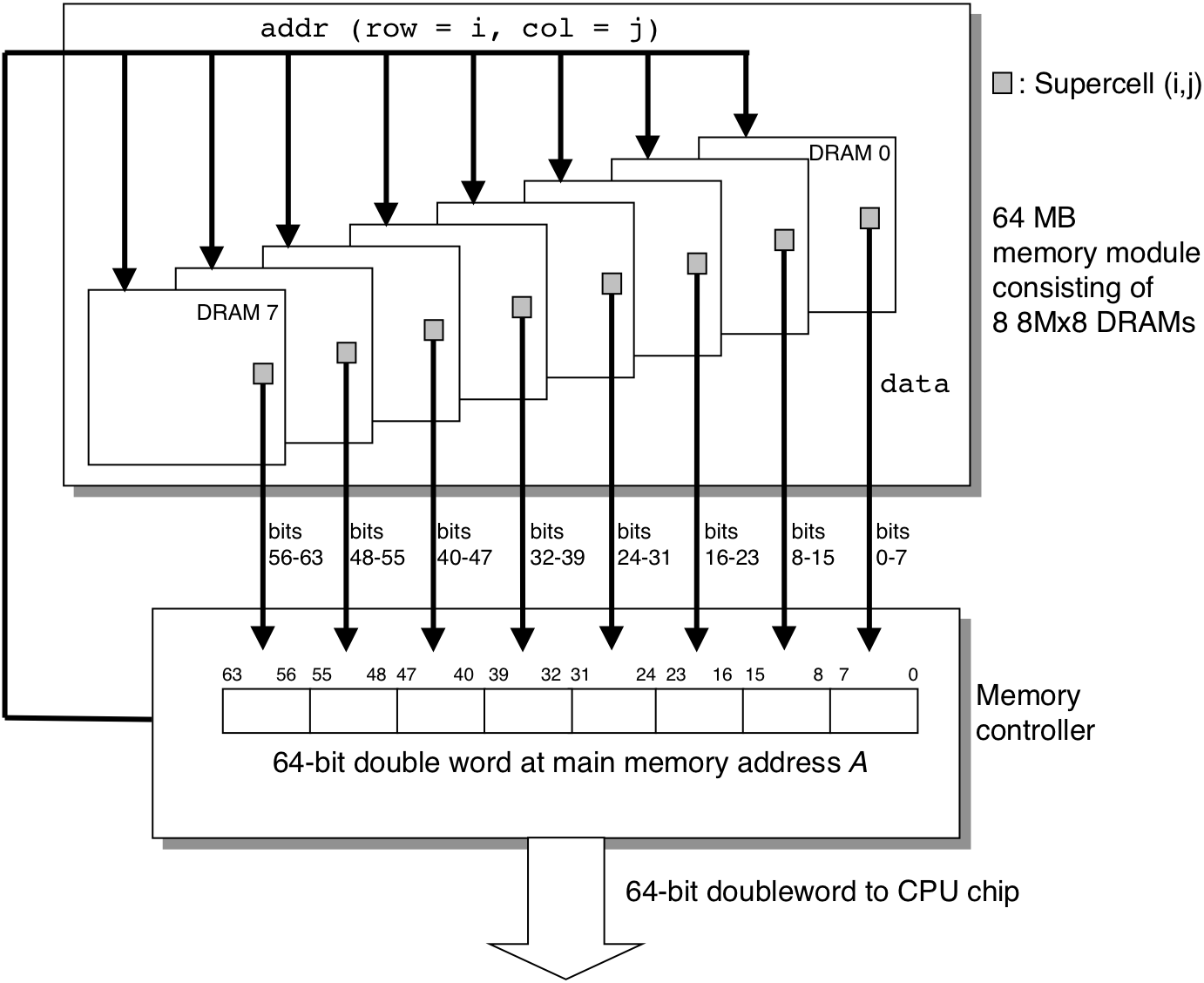
Figure 6.6: Typical bus structure that connects the CPU and main memory.
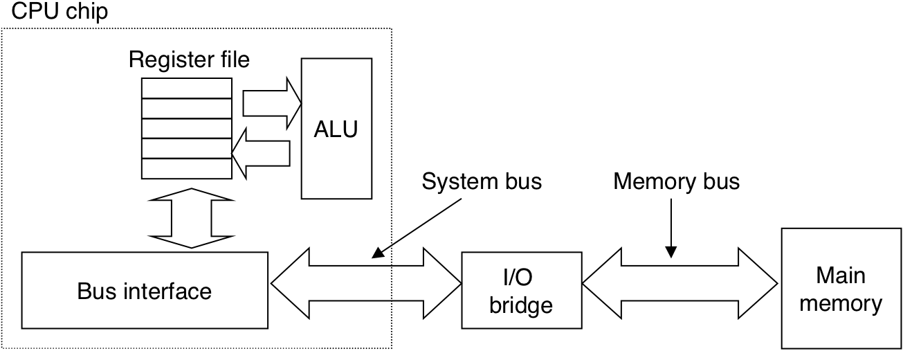
Figure 6.7: Memory read transaction for a load operation: movl A,%eax.
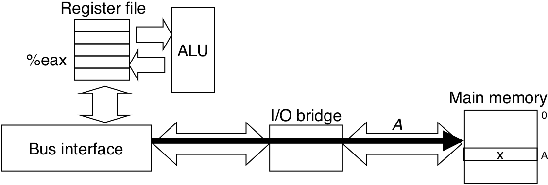
Figure 6.7: Memory read transaction for a load operation: movl A,%eax.
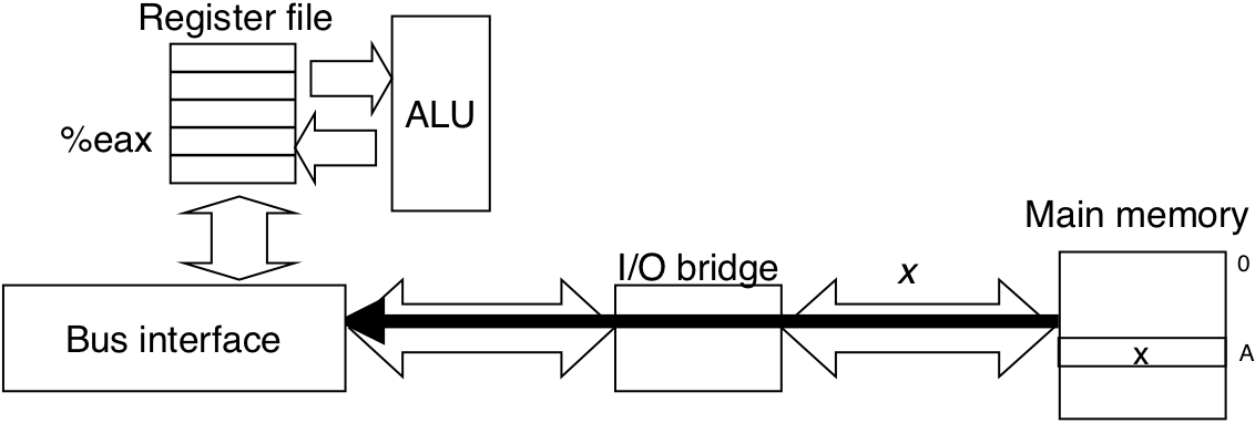
Figure 6.7: Memory read transaction for a load operation: movl A,%eax.
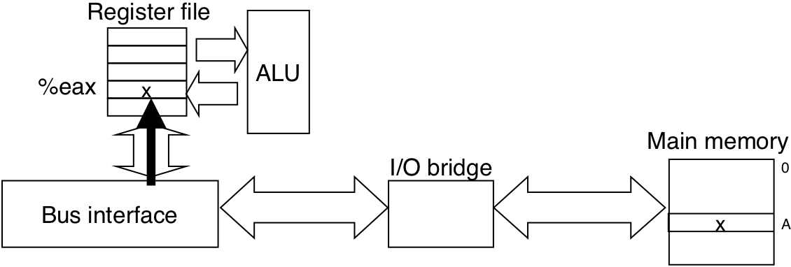
Figure 6.8: Memory write transaction for a store operation: movl %eax,A.
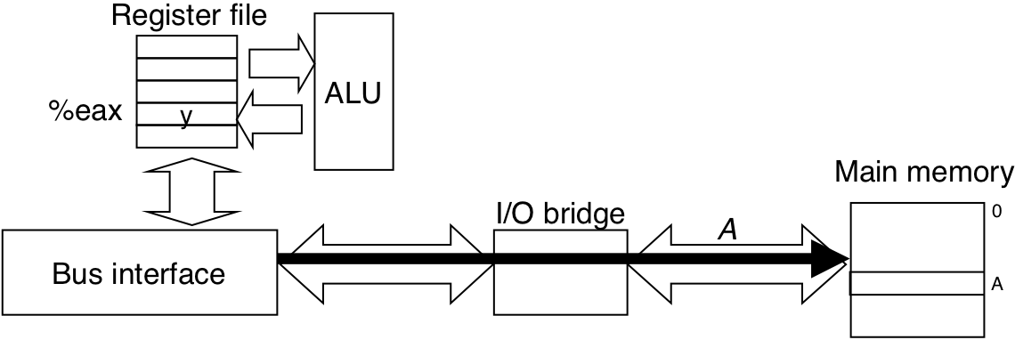
Figure 6.8: Memory write transaction for a store operation: movl %eax,A.
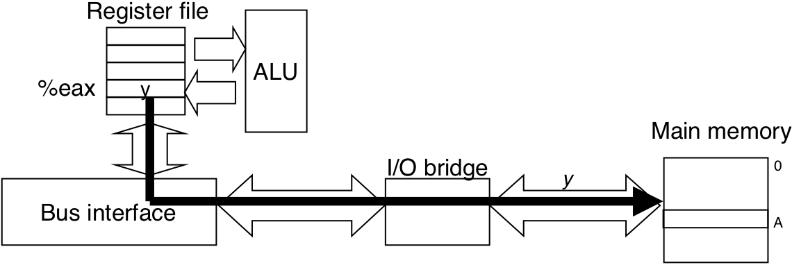
Figure 6.8: Memory write transaction for a store operation: movl %eax,A.
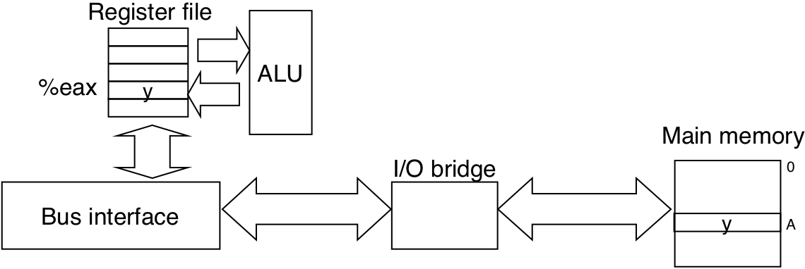
Figure 6.9: Disk geometry.
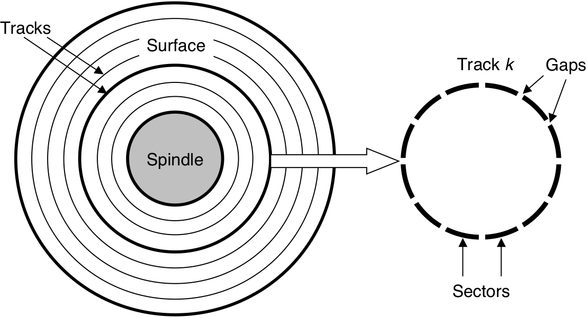
Figure 6.9: Disk geometry.
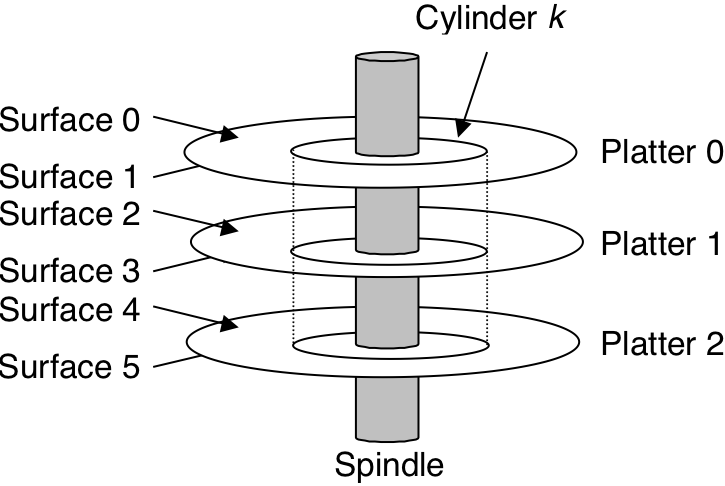
Figure 6.10: Disk dynamics.
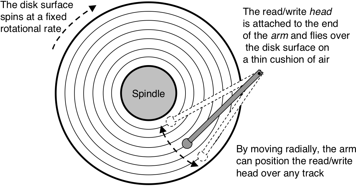
Figure 6.10: Disk dynamics.
Figure 6.11: Typical bus structure that connects the CPU, main memory, and I/O devices.
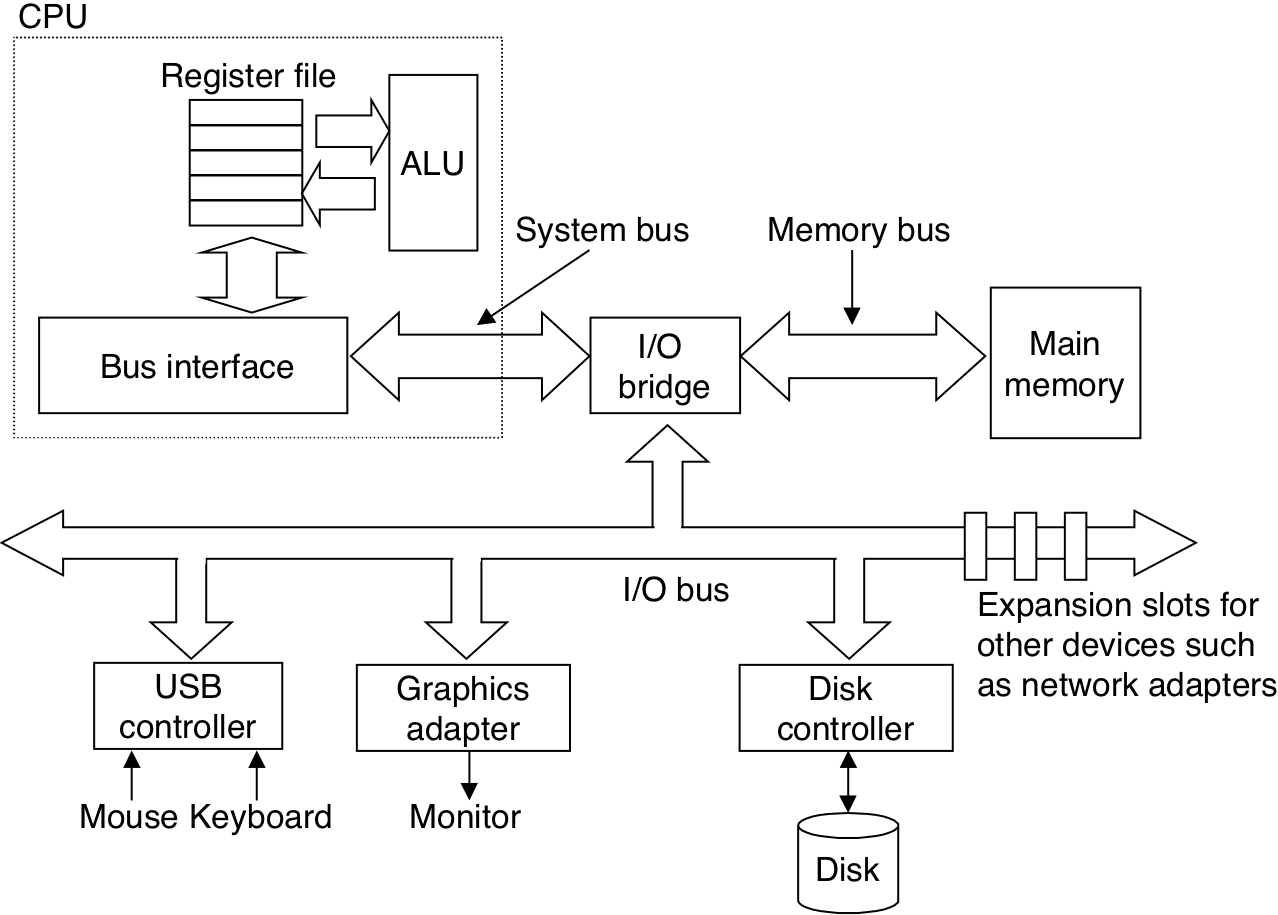
Figure 6.12: Reading a disk sector.
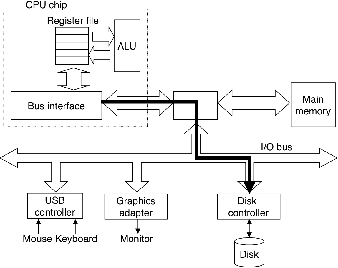
Figure 6.12: Reading a disk sector.
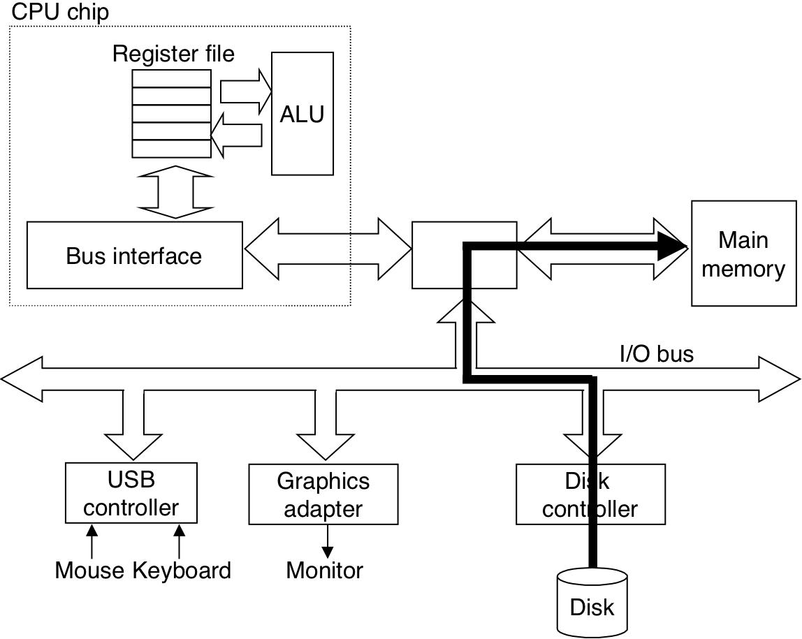
Figure 6.12: Reading a disk sector.
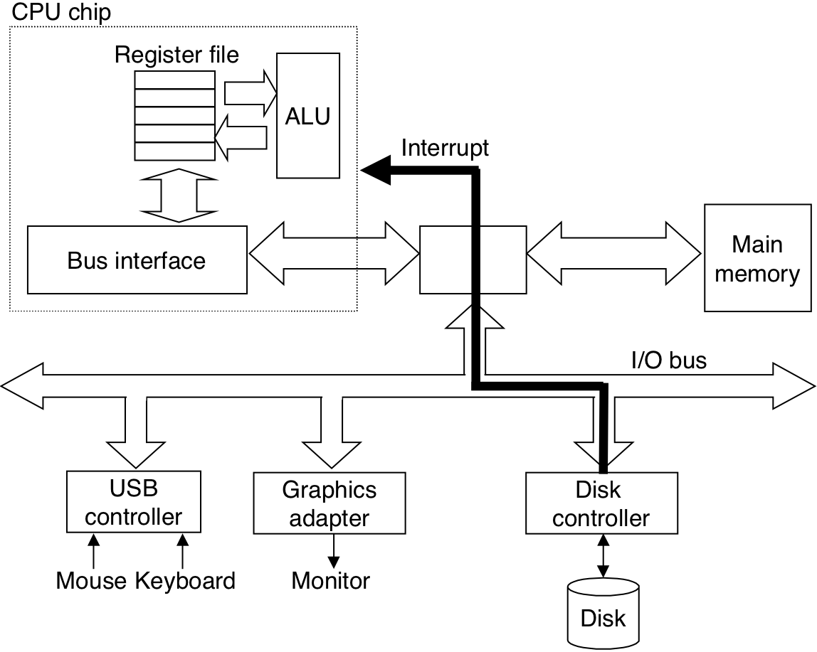
Figure 6.16: The increasing gap between DRAM, disk, and CPU speeds.
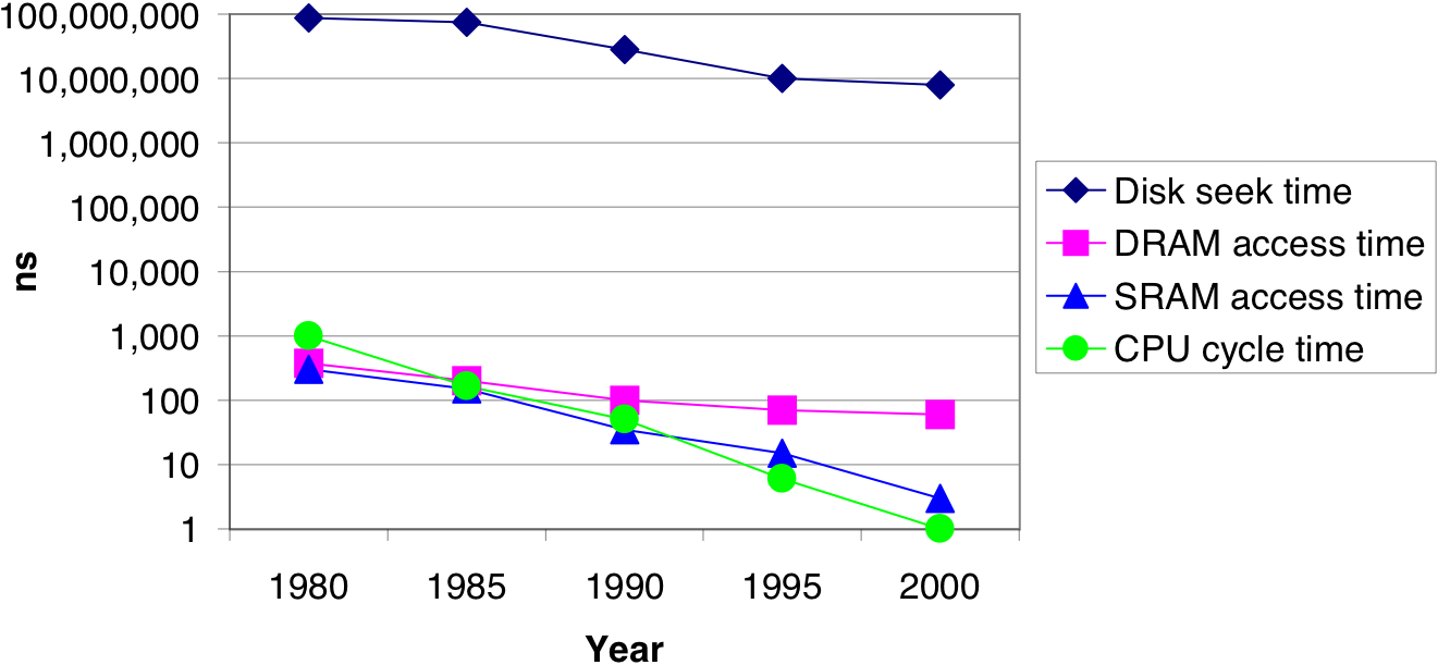
Figure 6.21: The memory hierarchy.

Figure 6.22: The basic principle of caching in a memory hierarchy.
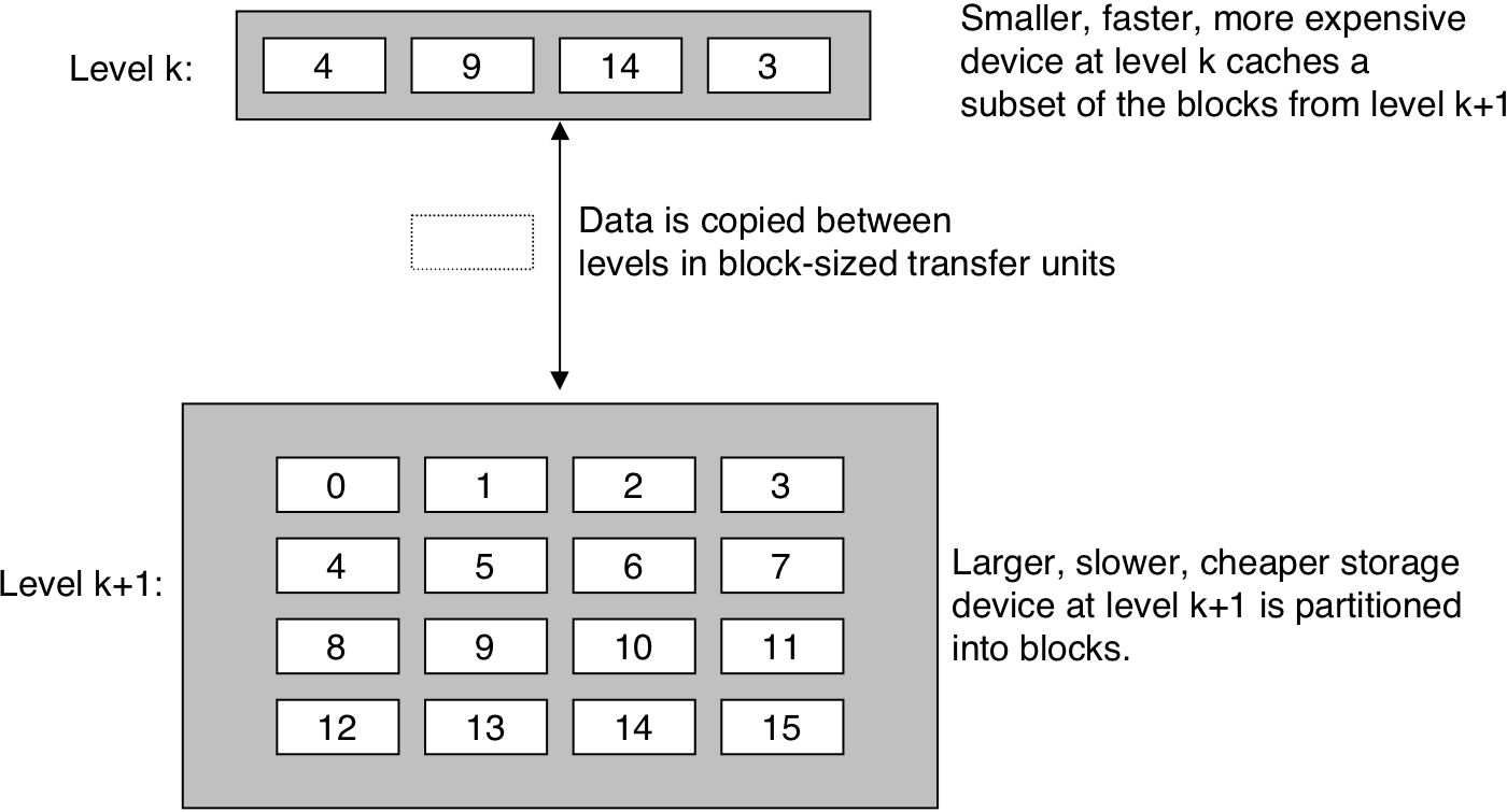
Figure 6.24: Typical bus structure for L1 and L2 caches.
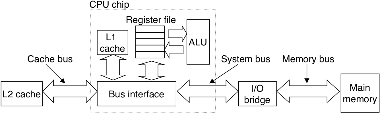
Figure 6.25: General organization of cache (S, E, B, m).
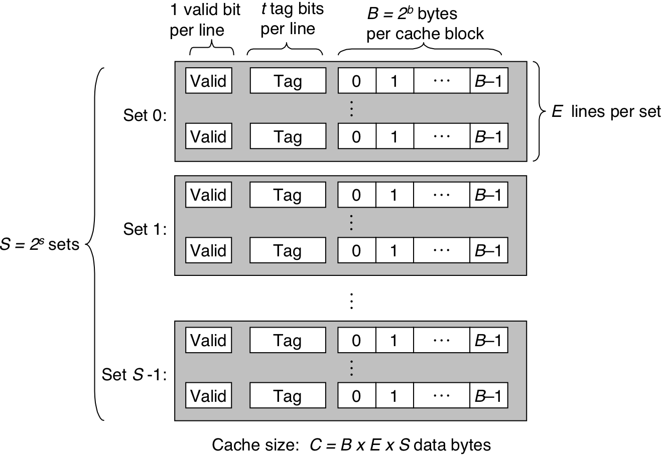
Figure 6.25: General organization of cache (S, E, B, m).
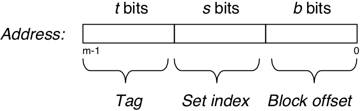
Figure 6.27: Direct-mapped cache (E = 1).
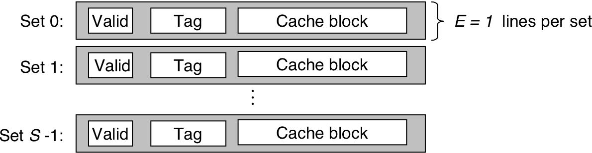
Figure 6.28: Set selection in a direct-mapped cache.
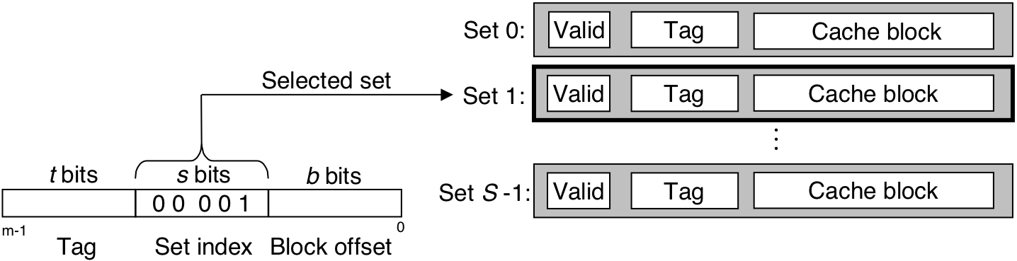
Figure 6.29: Line matching and word selection in a direct-mapped cache.
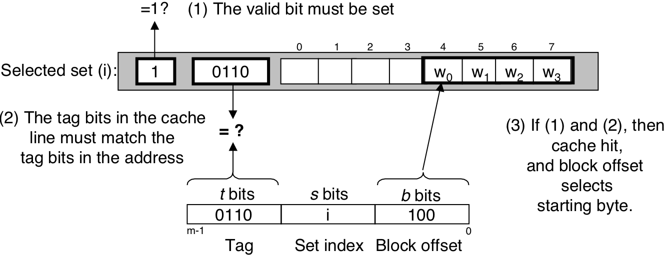
Figure 6.31: Why caches index with the middle bits.
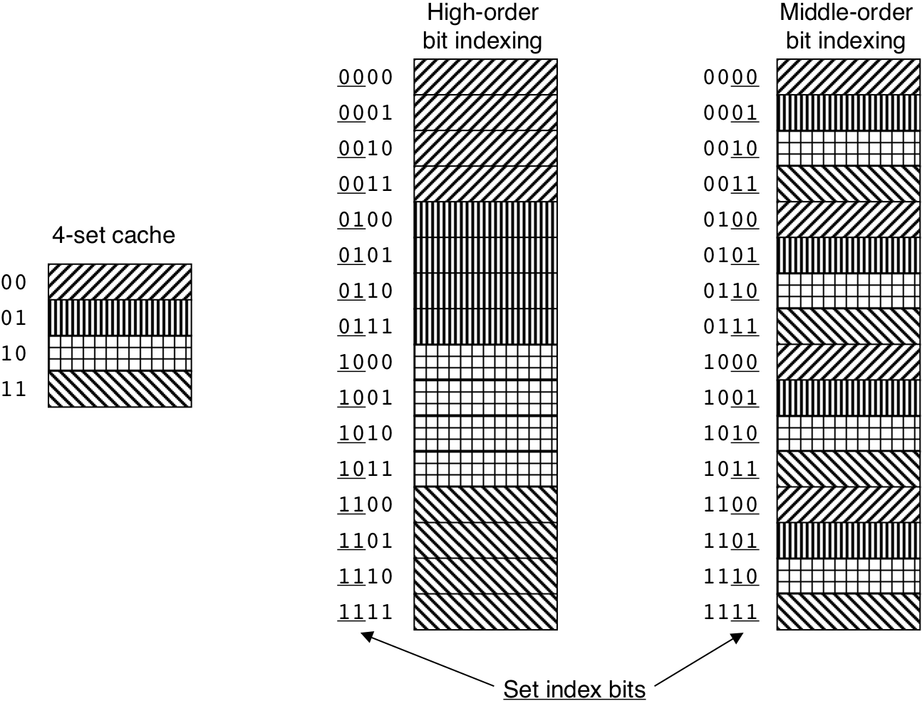
Figure 6.32: Set associative cache (1 < E < C/B).
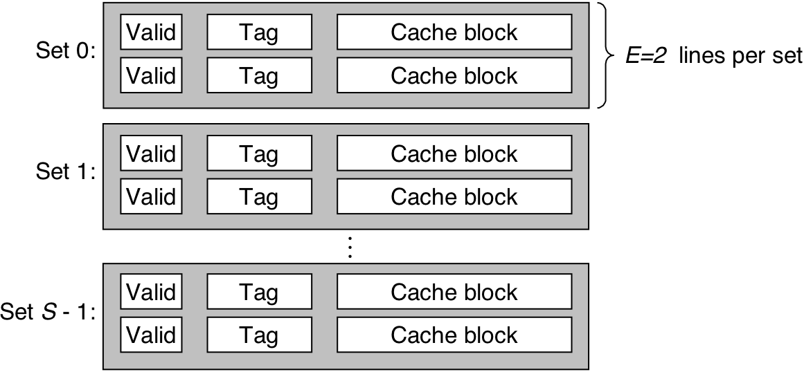
Figure 6.33: Set selection in a set associative cache.
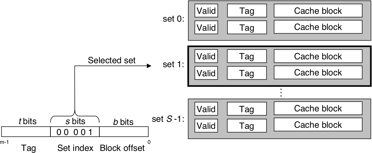
Figure 6.34: Line matching and word selection in a set associative cache.
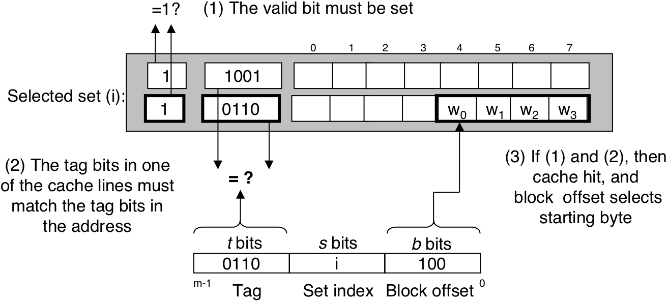
Figure 6.35: Fully set associative cache (E = C/B).
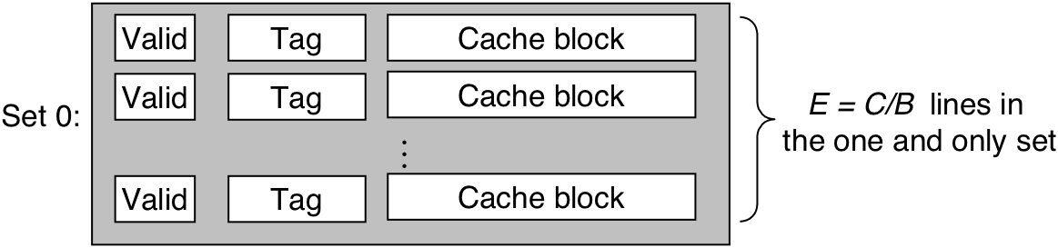
Figure 6.36: Set selection in a fully associative cache.
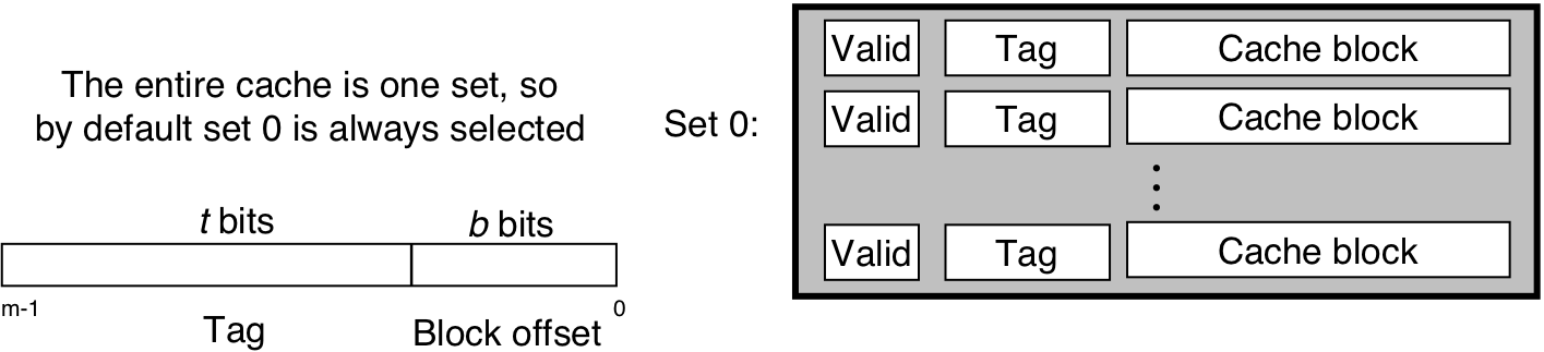
Figure 6.37: Line matching and word selection in a fully associative cache.
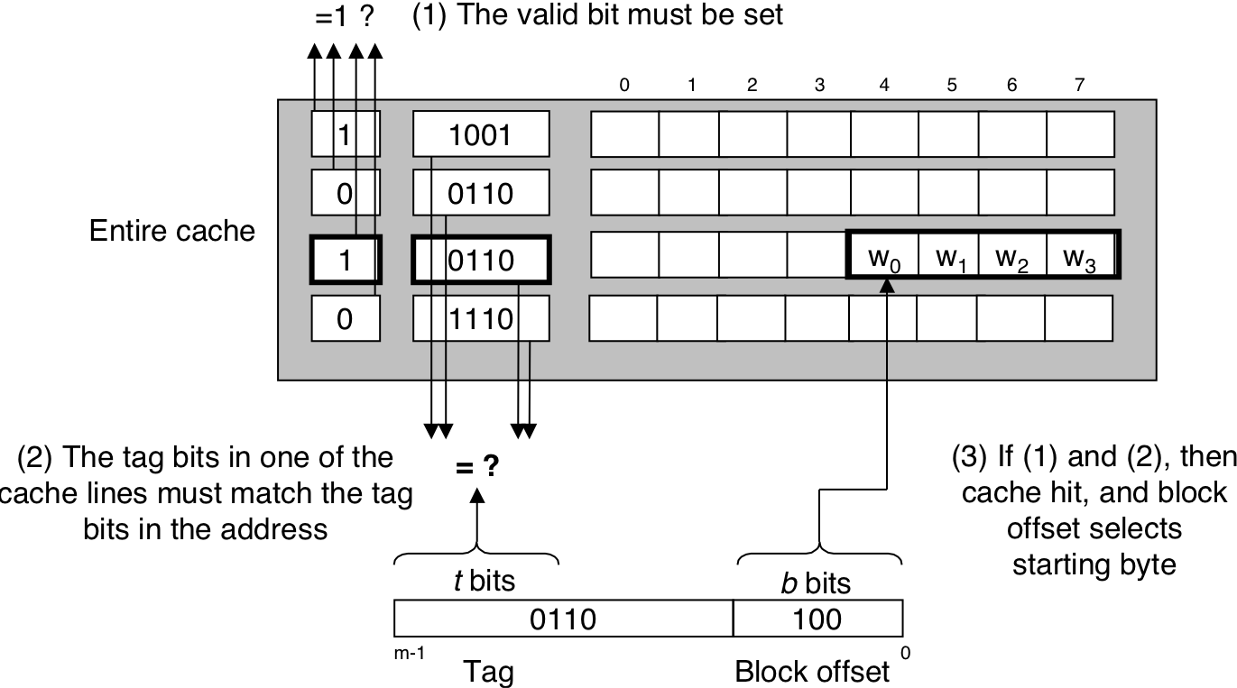
Figure 6.38: A typical multi-level cache organization.
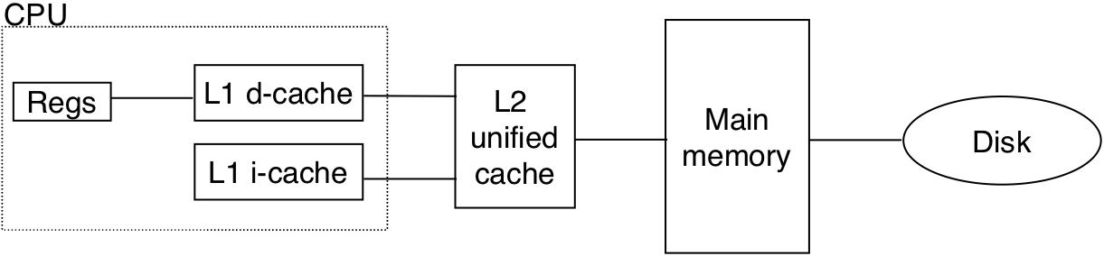
Figure 6.42: The memory mountain.
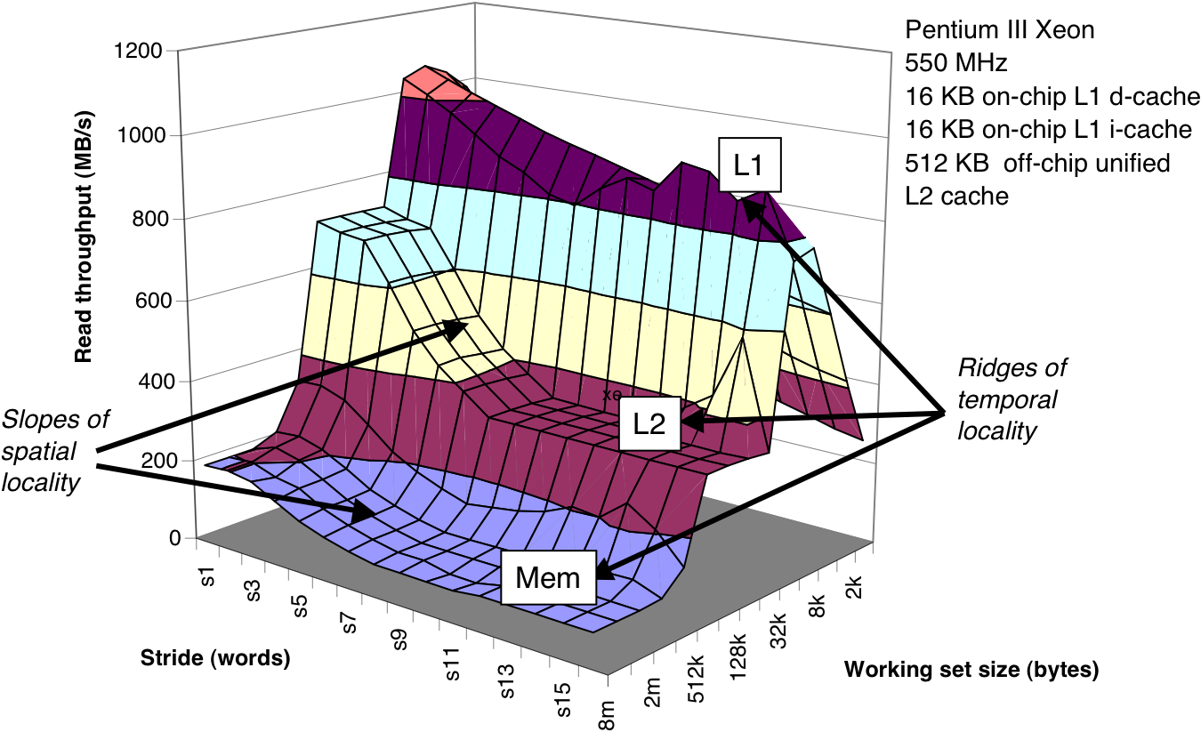
Figure 6.43: Ridges of temporal locality in the memory mountain.
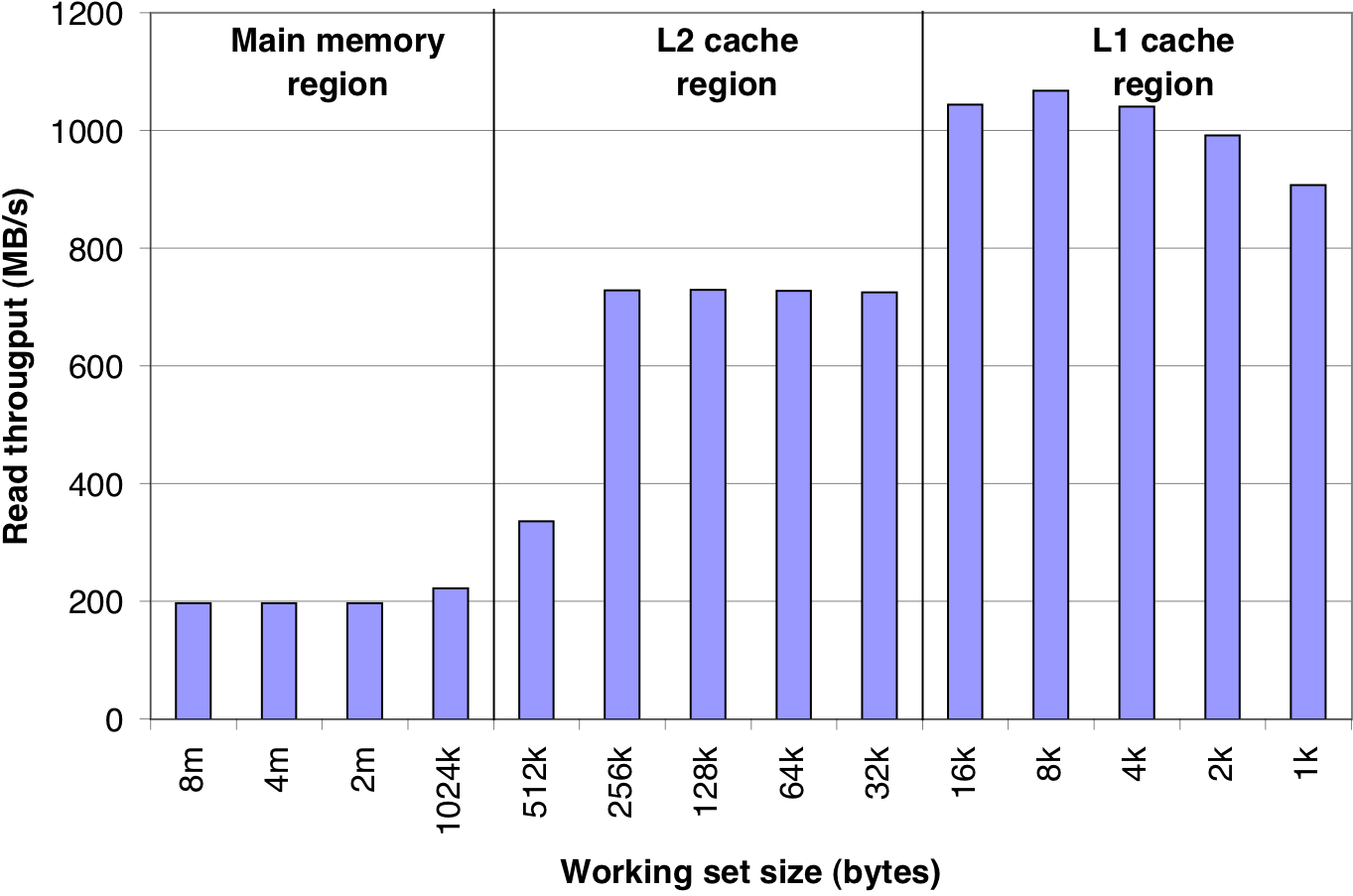
Figure 6.44: A slope of spatial locality.
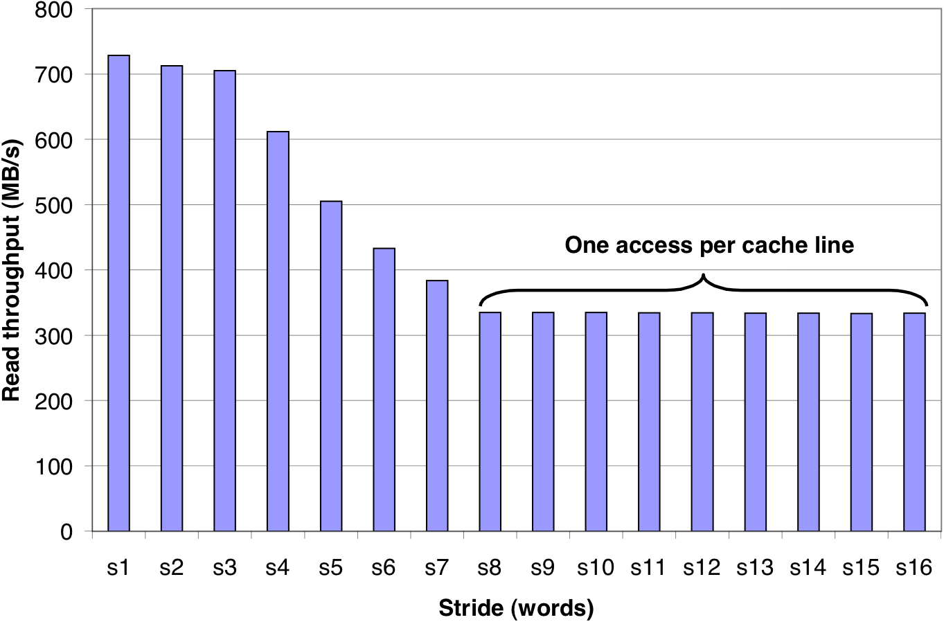
Figure 6.47: Pentium III Xeon matrix multiply performance.
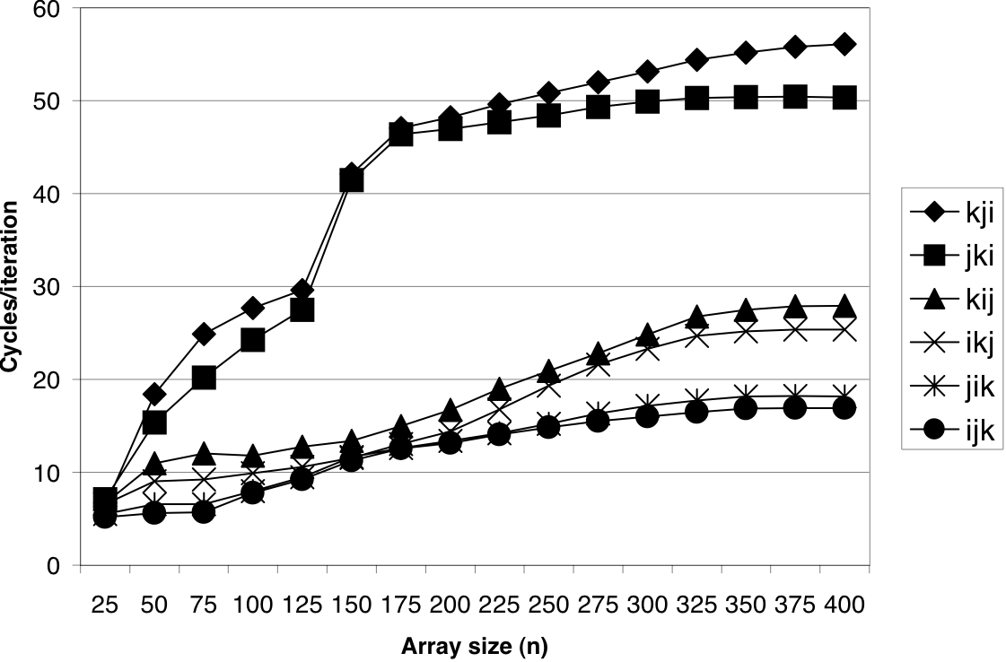
Figure 6.49: Graphical interpretation of blocked matrix multiply
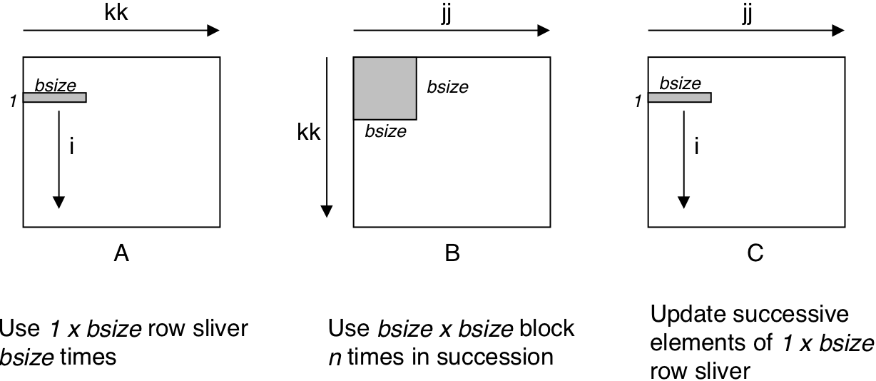
Figure 6.50: Pentium III Xeon blocked matrix multiply performance.
| 7 [7/13] |
Figure 7.2: Static linking.
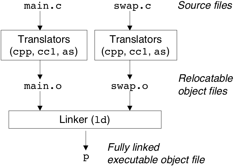
Figure 7.3: Typical ELF relocatable object file.
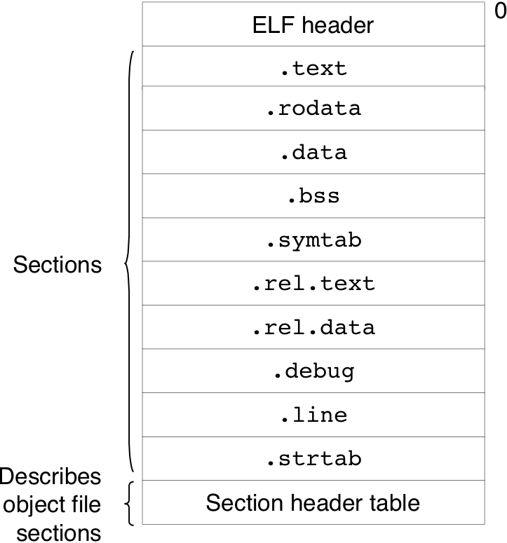
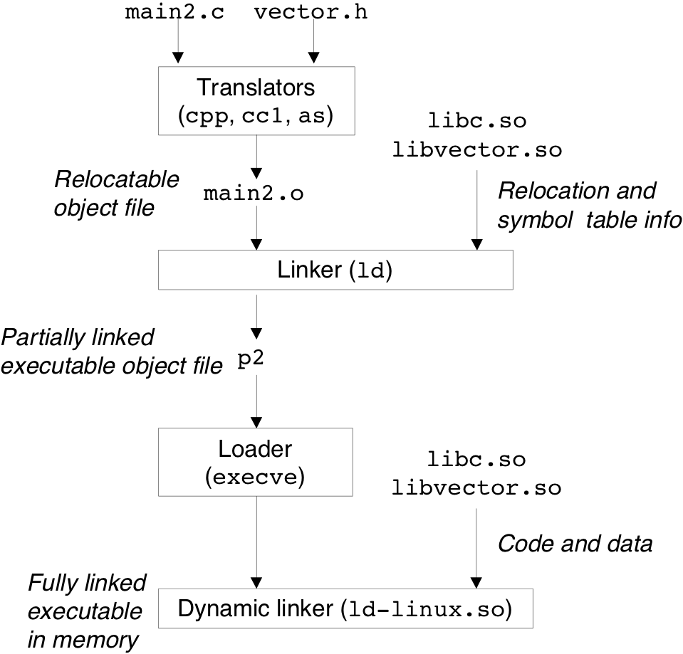
Figure 7.7: Linking with static libraries.

Figure 7.11: Typical ELF executable object file
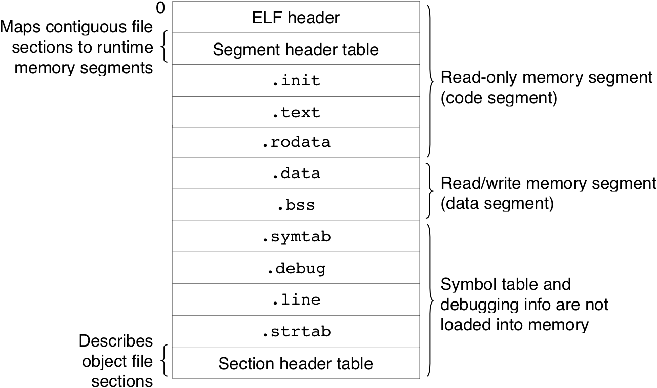
Figure 7.13: Linux run-time memory image
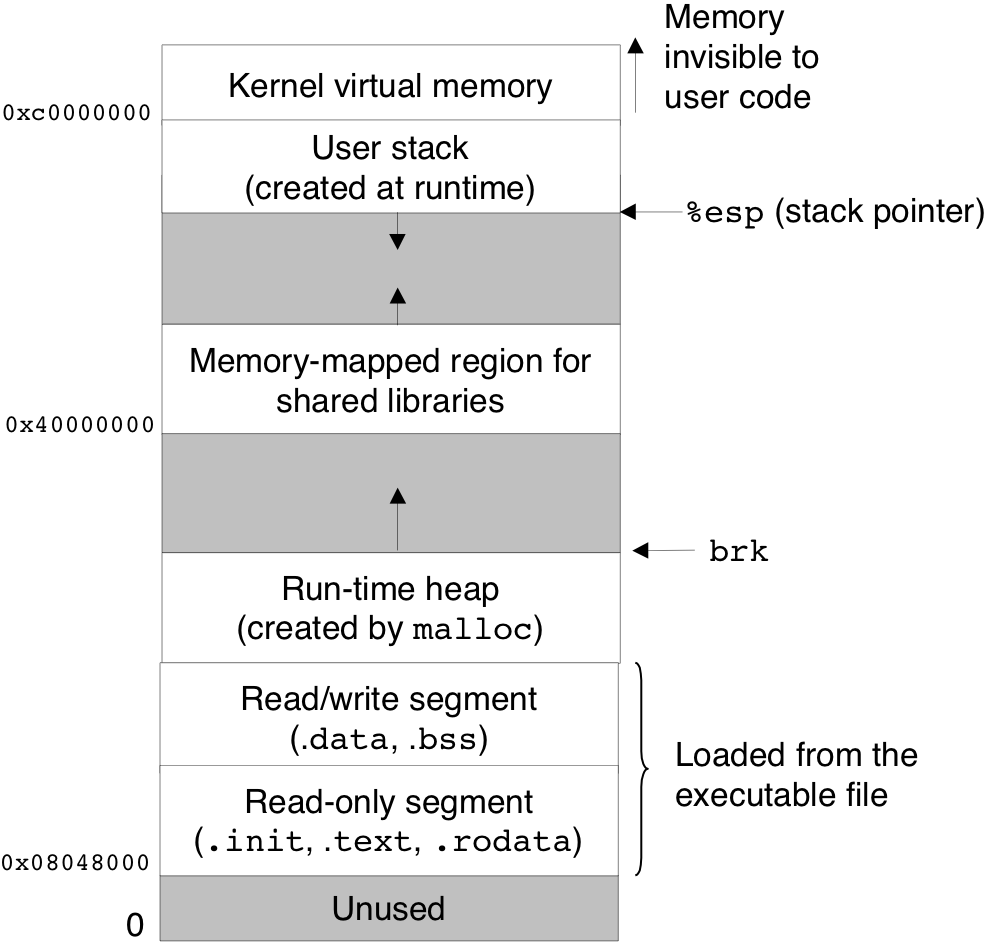
Figure 7.15: Dynamic linking with shared libraries.
| 8 [8/13] |
Figure 8.1: Anatomy of an exception.
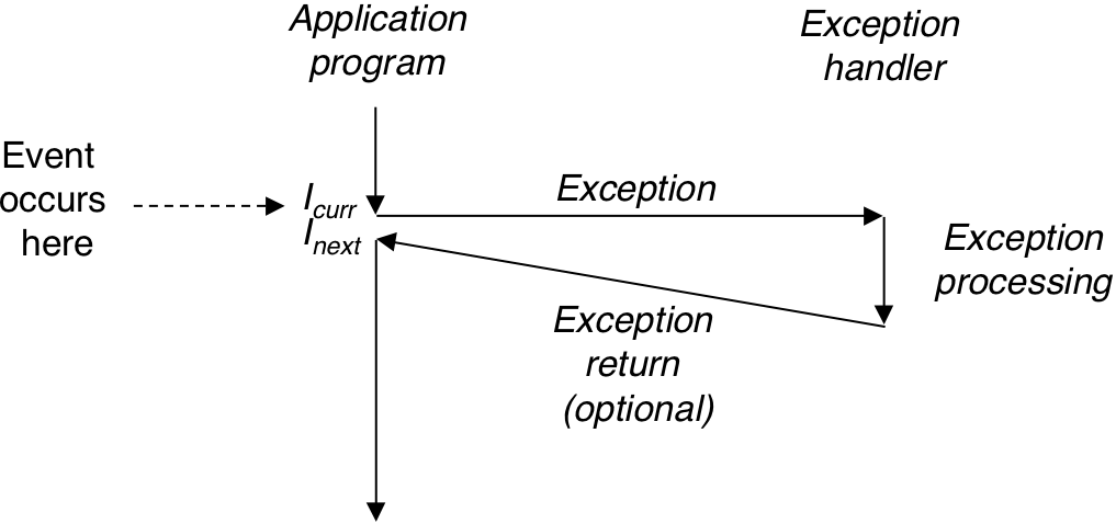
Figure 8.2: Exception table.
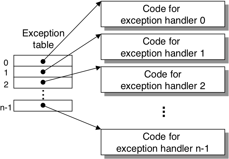
Figure 8.3: Generating the address of an exception handler.
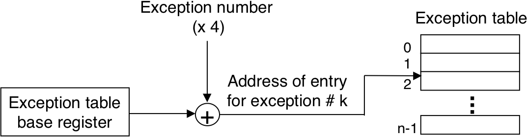
Figure 8.5: Interrupt handling.
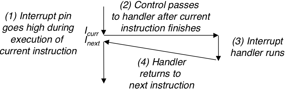
Figure 8.6: Trap handling.
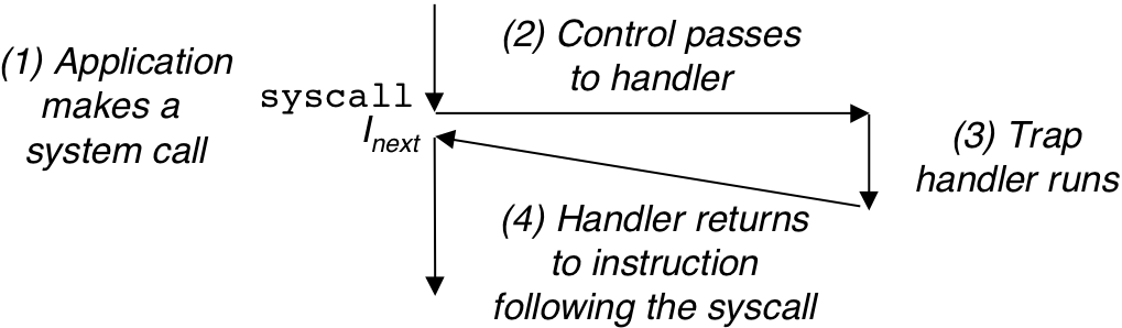
Figure 8.7: Fault handling.
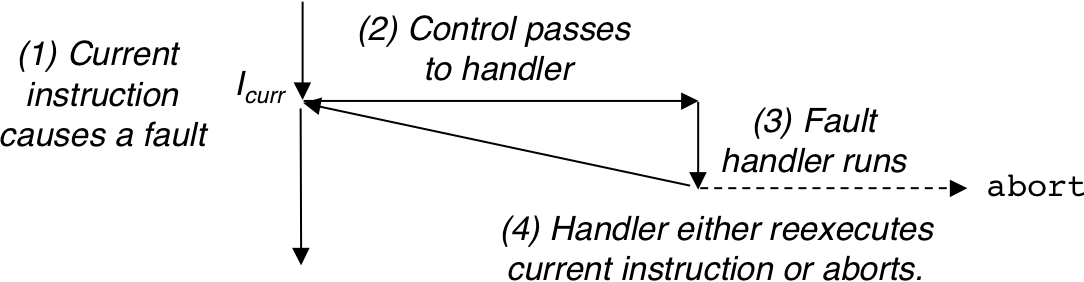
Figure 8.8: Abort handling.
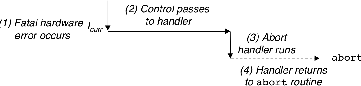
Figure 8.10: Logical control flows.
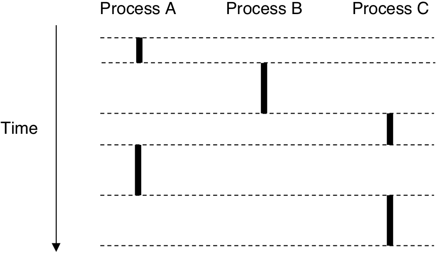
Figure 8.11: Process address space.
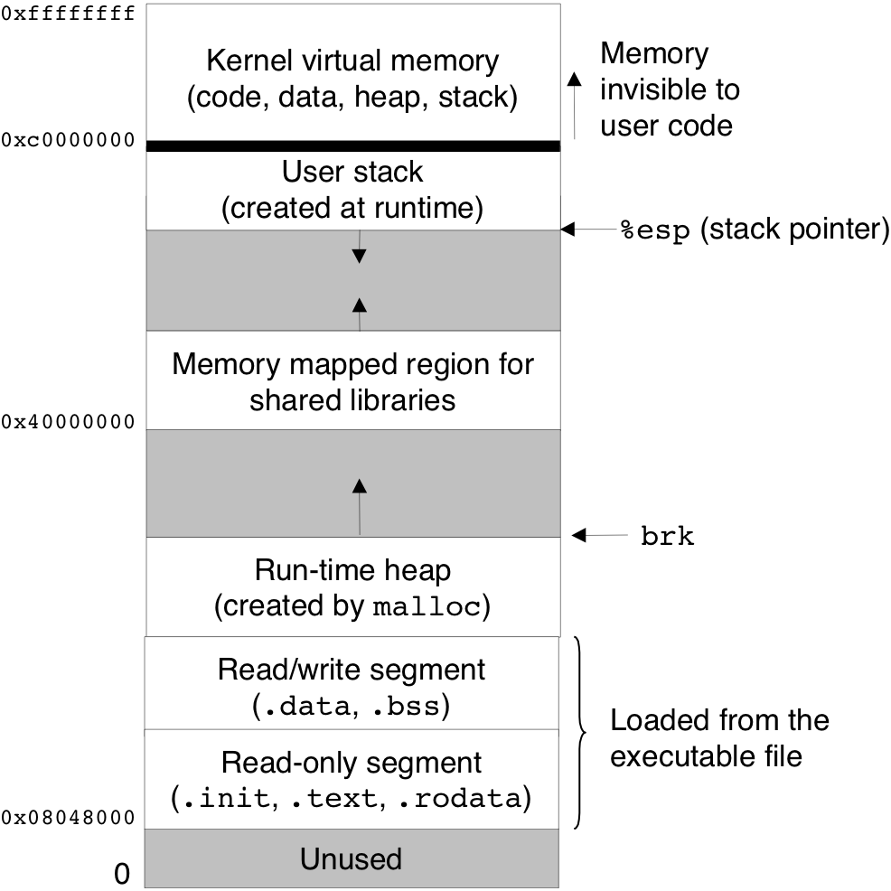
Figure 8.12: Anatomy of a process context switch.
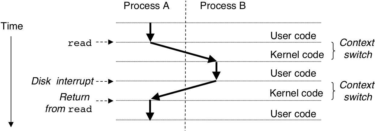
Figure 8.14: Examples of fork programs.
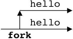
Figure 8.14: Examples of fork programs.
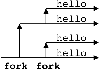
Figure 8.14: Examples of fork programs.
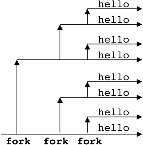
Figure 8.17: Organization of an argument list.
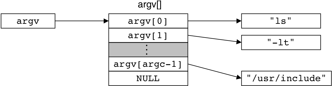
Figure 8.18: Organization of an environment variable list.
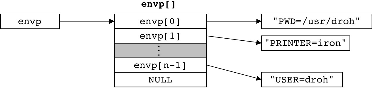
Figure 8.19: Typical organization of the user stack when a new program starts.
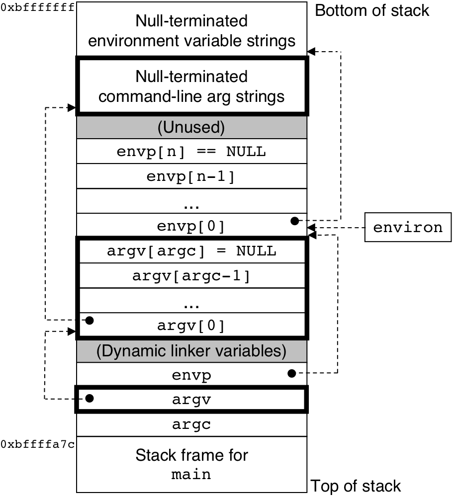
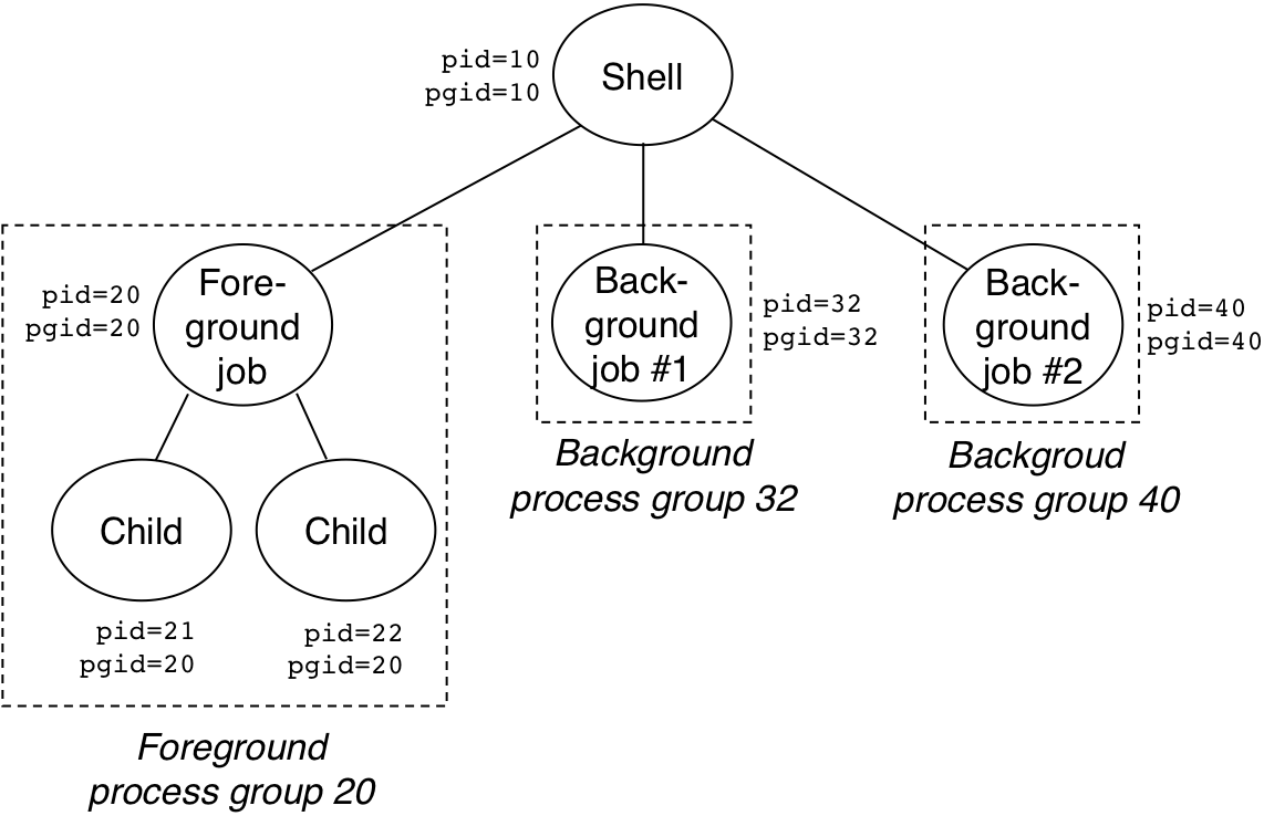
Figure 8.24: Foreground and background process groups.
| 9 [9/13] |
Figure 9.1: Time scale of computer system events.
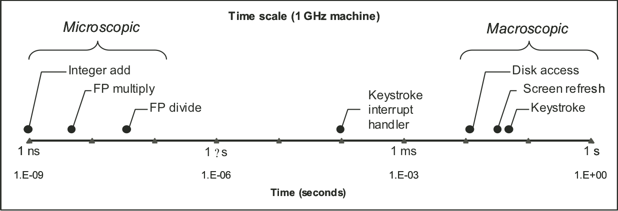
Figure 9.2: System's vs.~applications view of time.
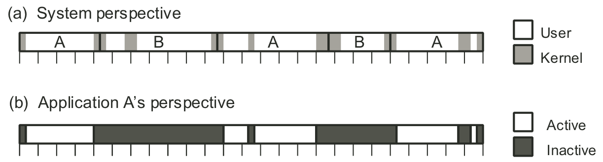
Figure 9.4: Graphical representation of trace in Figure ....
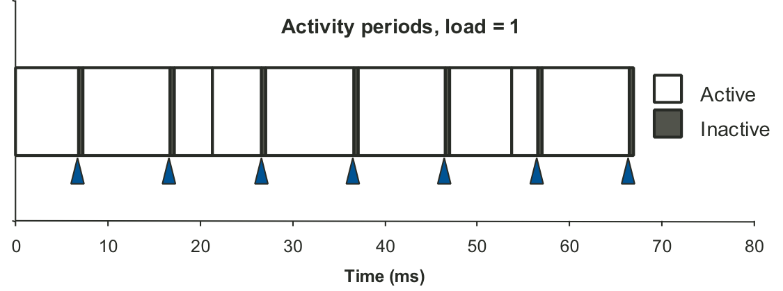
Figure 9.6: Graphical representation of activity periods for trace in Figure ....
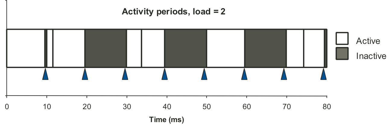
Figure 9.7: Process timing by interval counting.
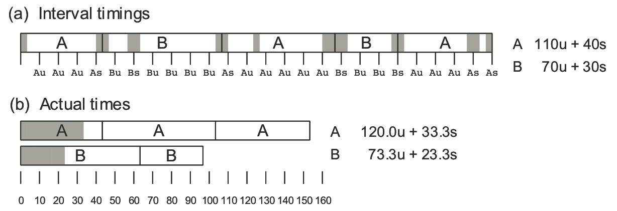
Figure 9.8: Measuring interval counting accuracy.
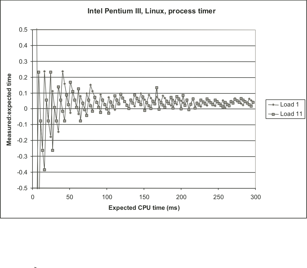
Figure 9.11: Measurements of long duration procedure under different loading conditions.
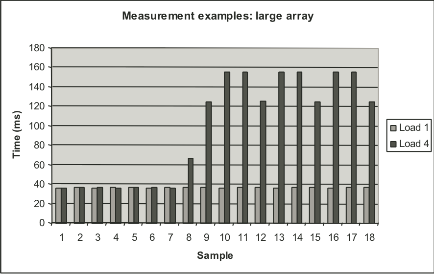
Figure 9.12: measurements of short duration procedure under different loading conditions.
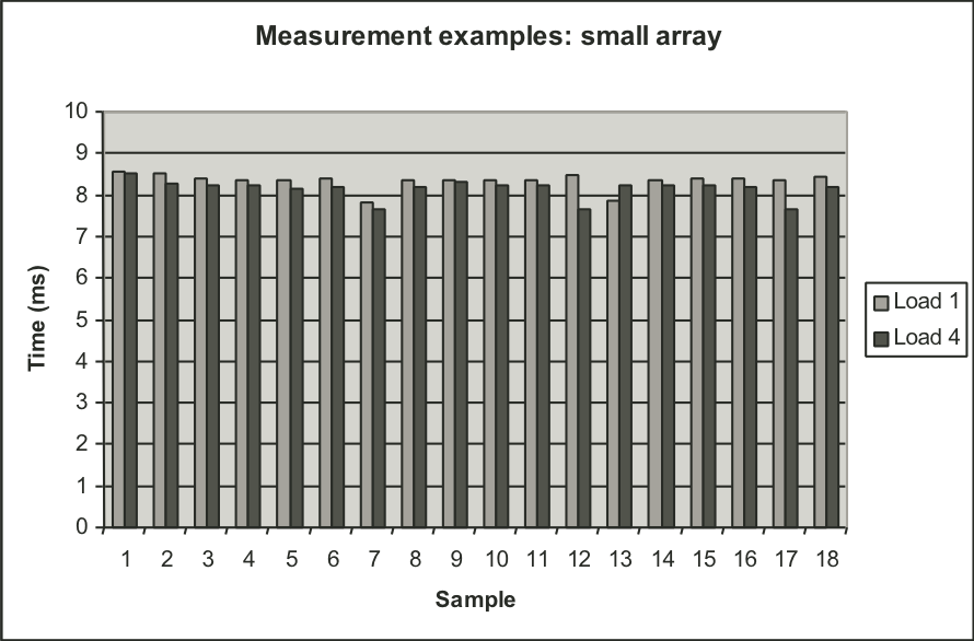
Figure 9.14: Experimental validation of K-best measurement scheme on Linux system
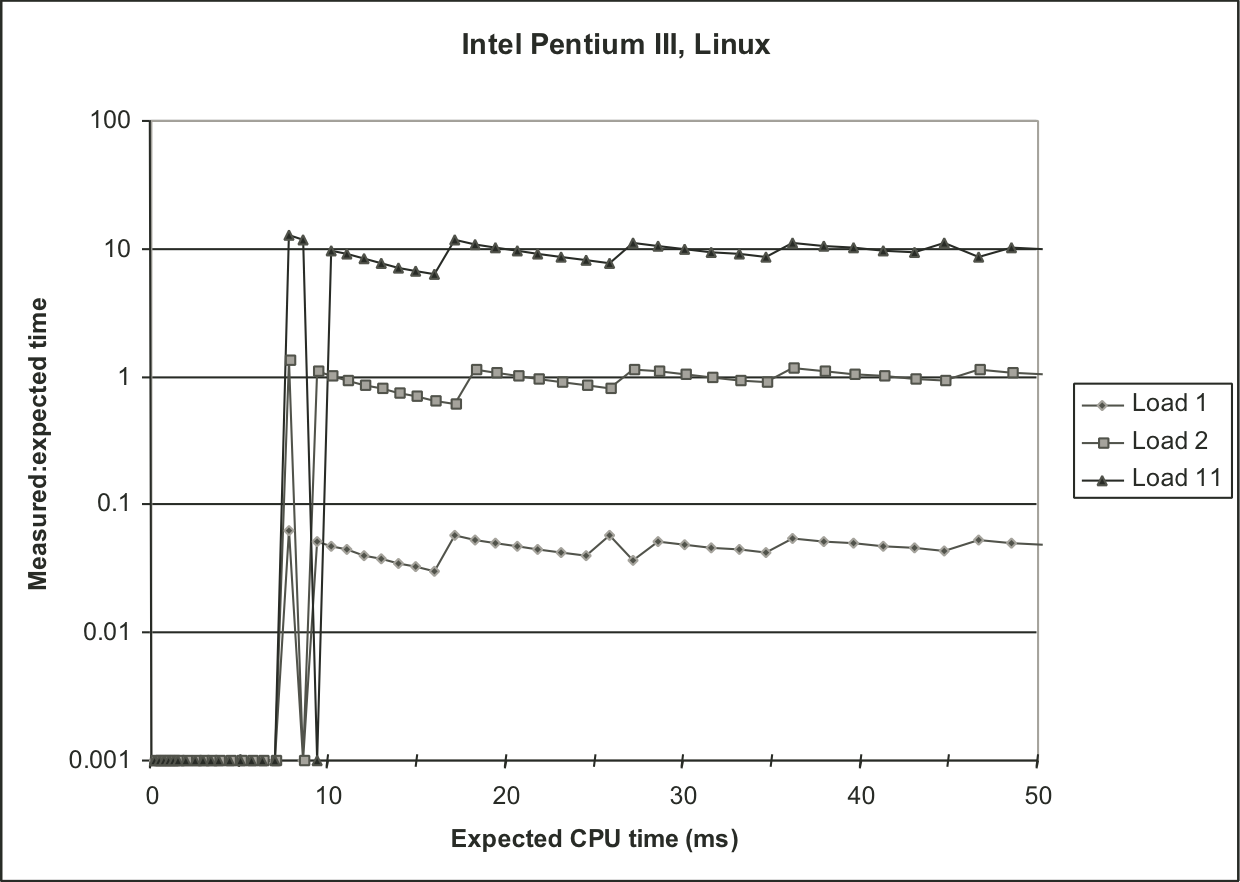
Figure 9.15: Effectiveness of K-best scheme for different values of K.
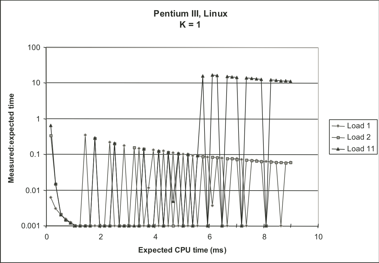
Figure 9.15: Effectiveness of K-best scheme for different values of K.
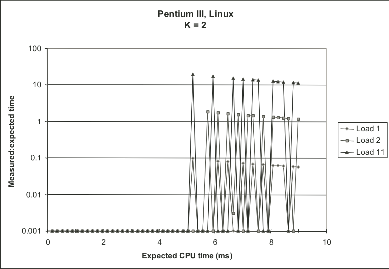
Figure 9.15: Effectiveness of K-best scheme for different values of K.
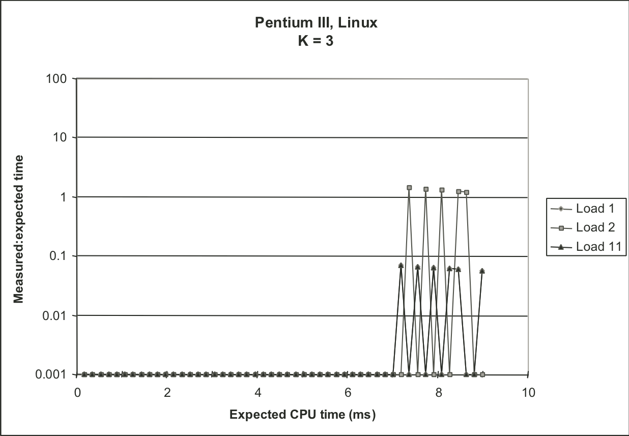
Figure 9.15: Effectiveness of K-best scheme for different values of K.
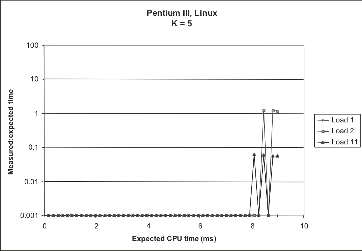
Figure 9.16: Measurements with compensation for timer interrupt overhead.
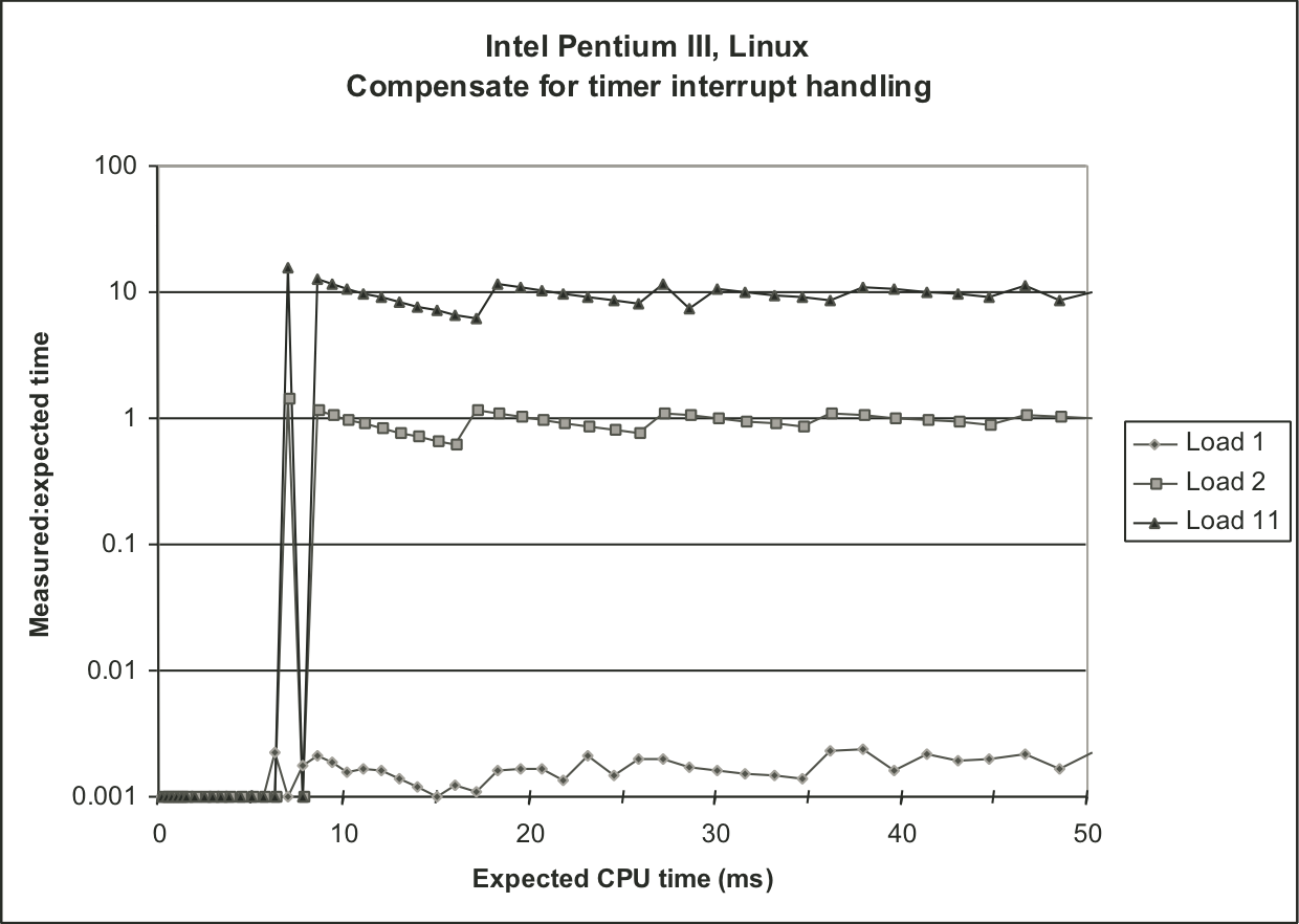
Figure 9.17: Experimental validation of K-best measurement scheme on IA32/Linux system with older version of the kernel.
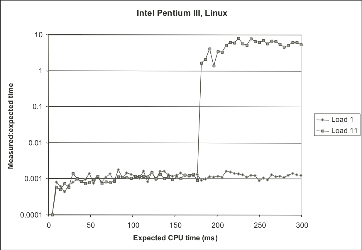
Figure 9.18: Experimental validation of K-best measurement scheme on Windows-NT system.
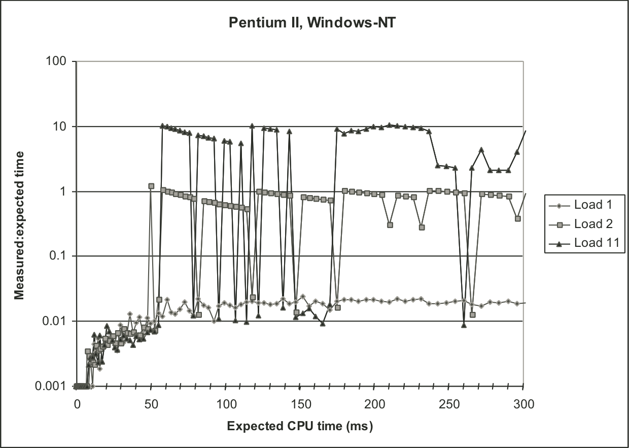
Figure 9.19: Experimental validation of K-best measurement scheme on Compaq Alpha system.
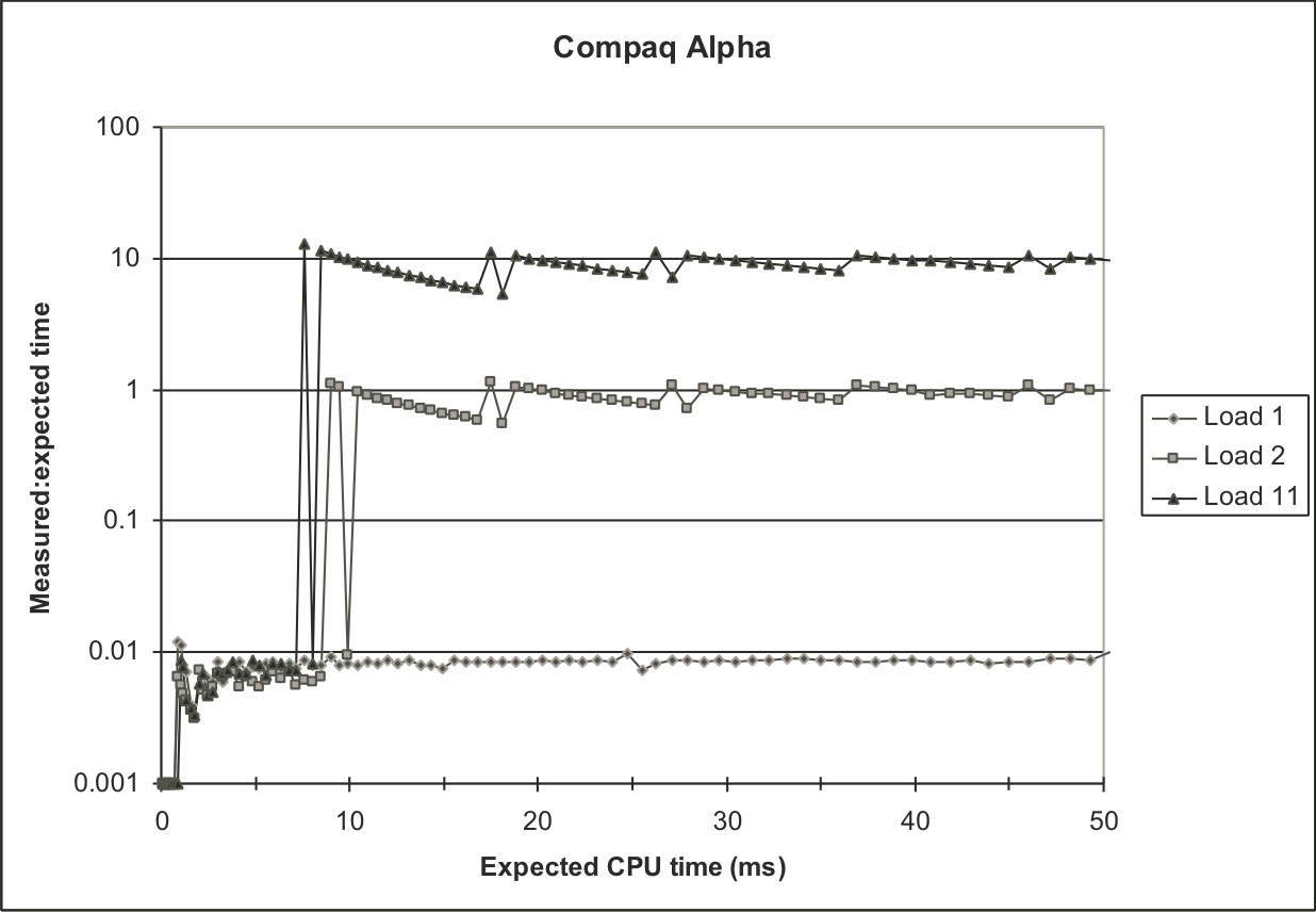
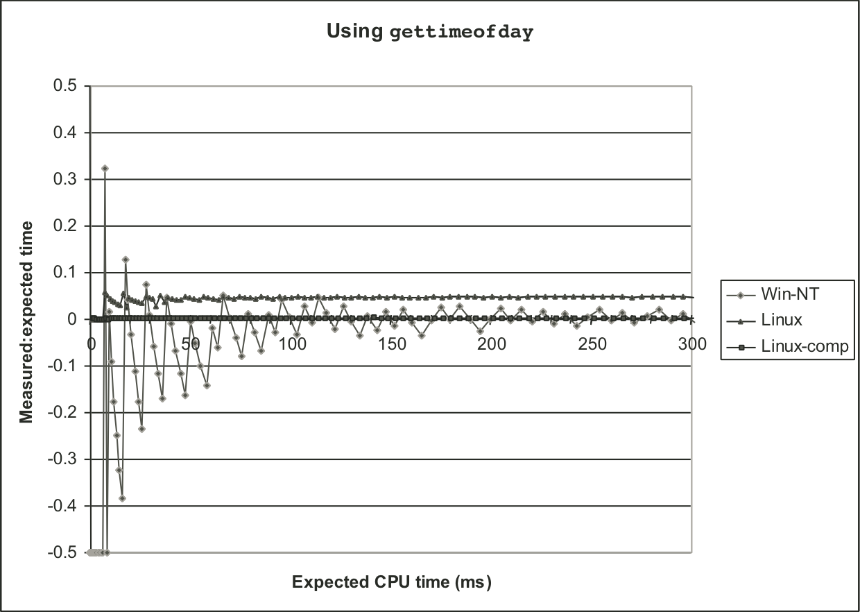
Figure 9.22: Experimental validation of K-best measurement scheme using gettimeofday function.
| 10 [10/13] |
Figure 10.1: A system that uses physical addressing.
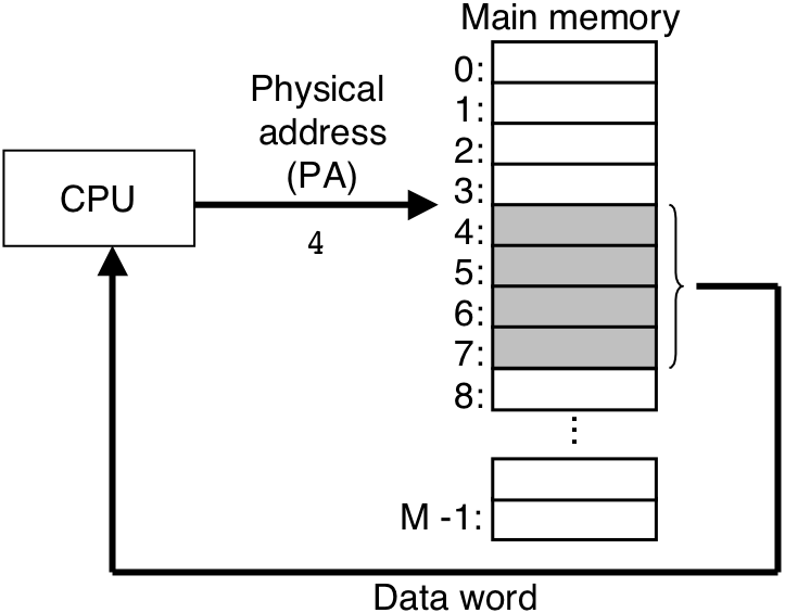
Figure 10.2: A system that uses virtual addressing.
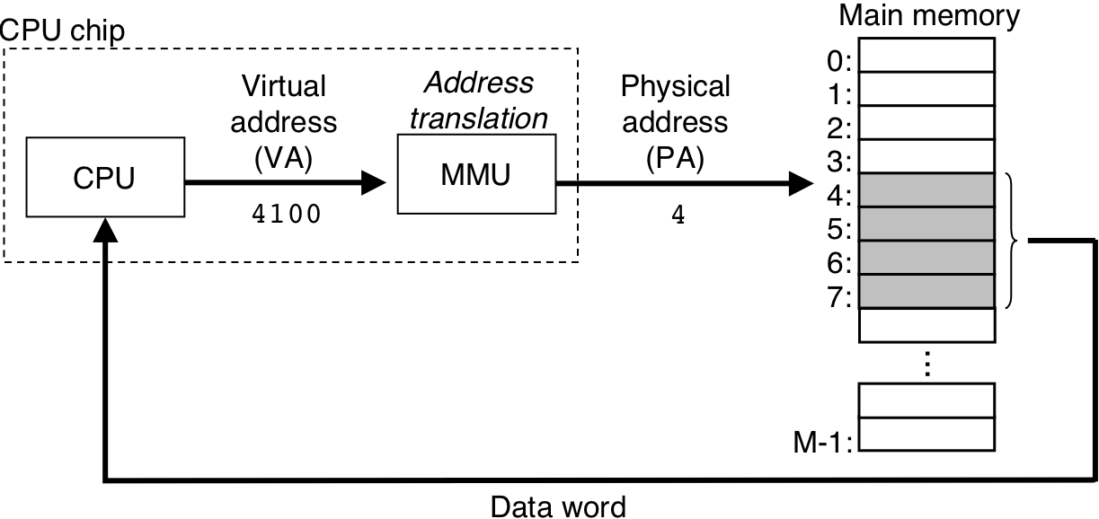
Figure 10.3: How a VM system uses main memory as a cache.
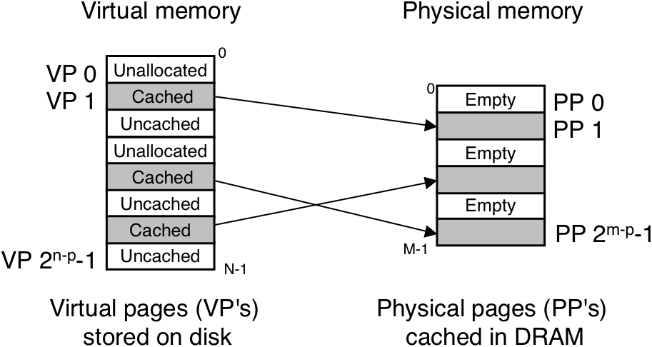
Figure 10.4: Page table.
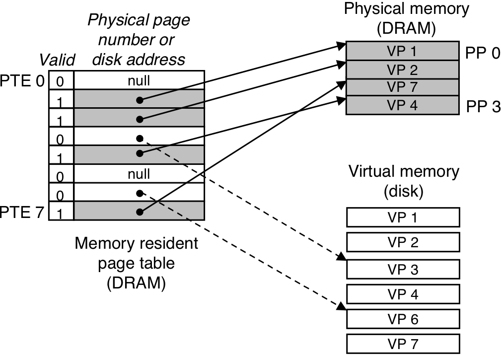
Figure 10.5: VM page hit.
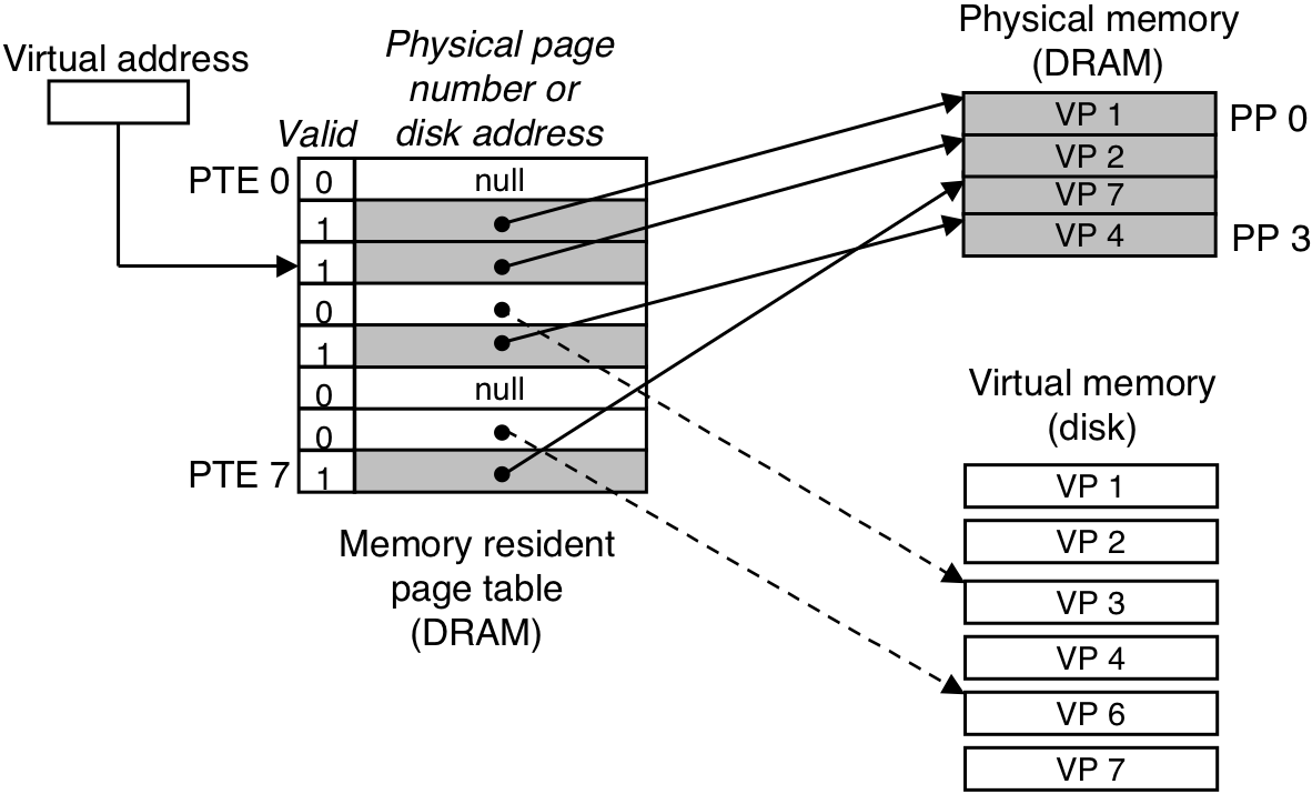
Figure 10.6: VM page fault (before).
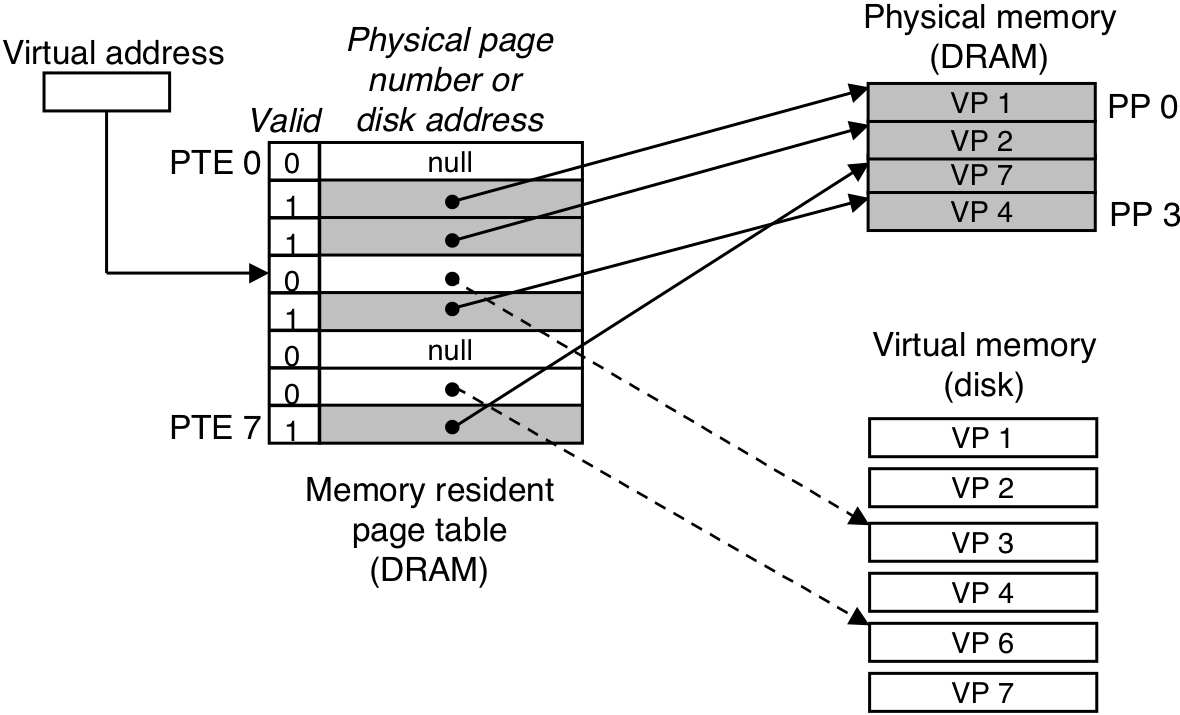
Figure 10.7: VM page fault (after).
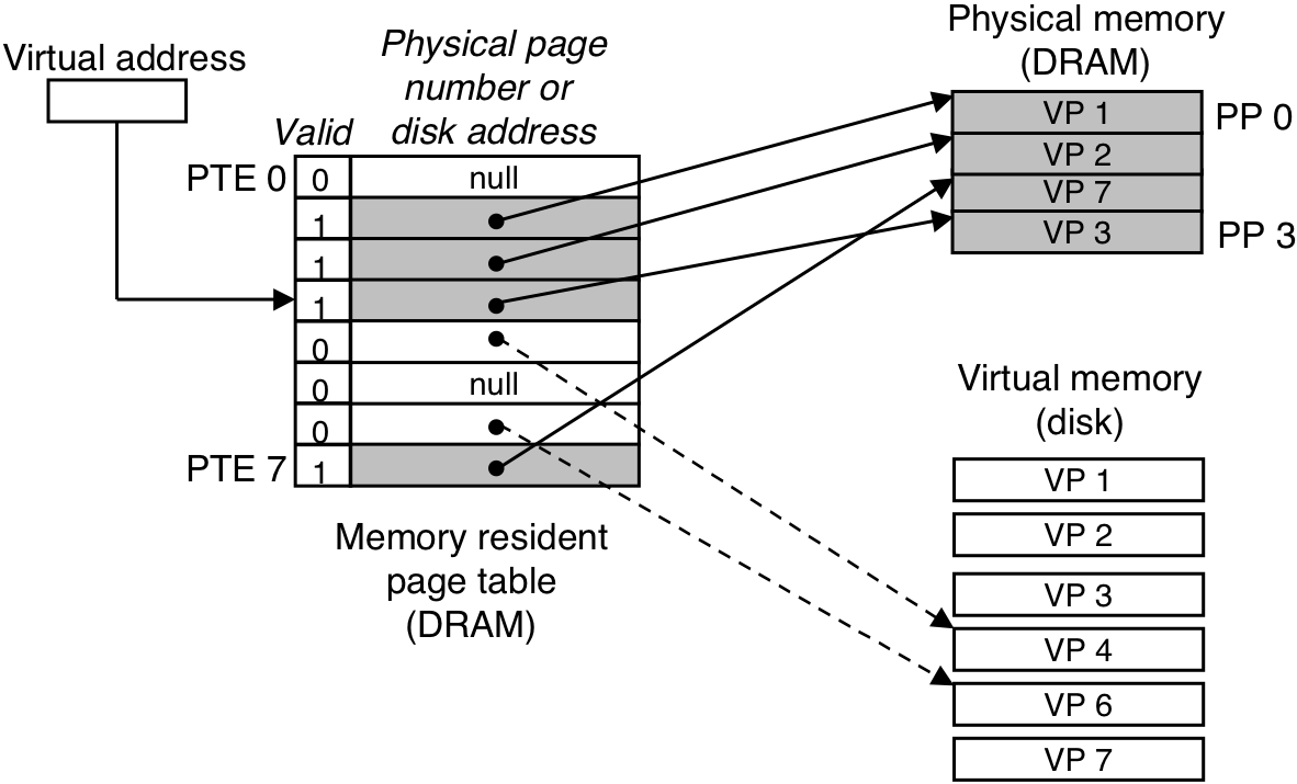
Figure 10.8: Allocating a new virtual page.
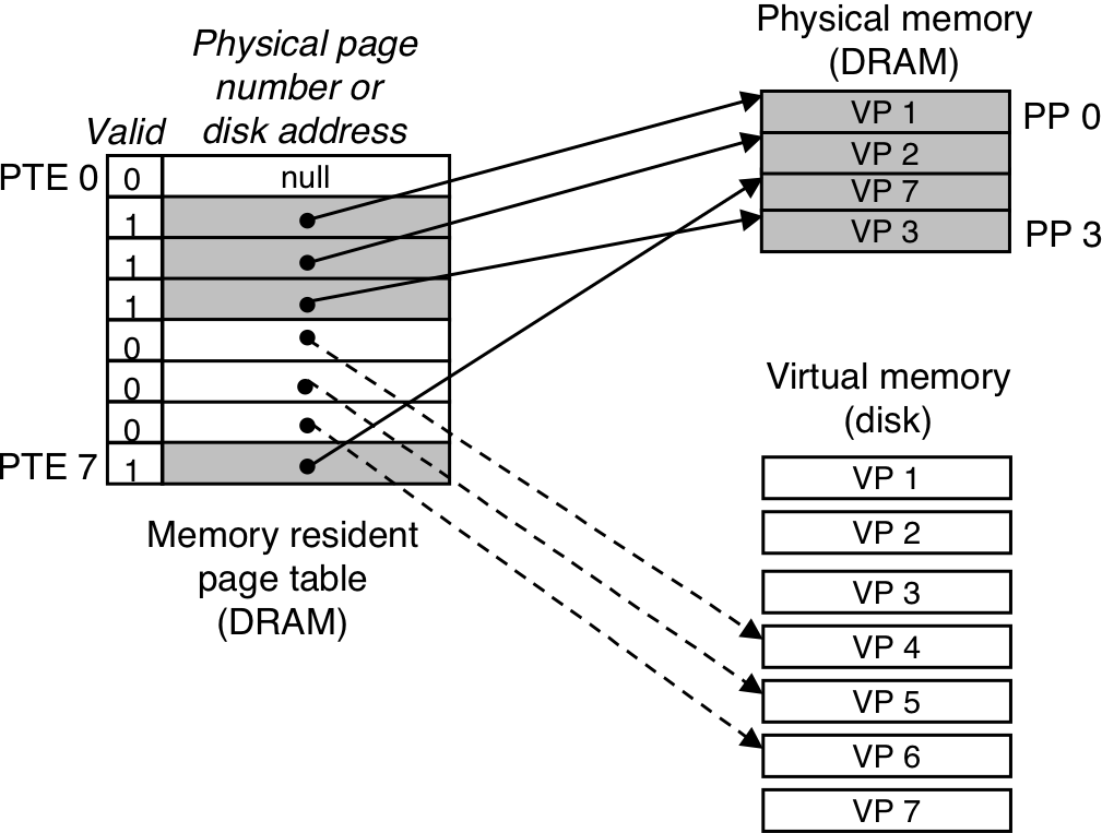
Figure 10.9: How VM provides processes with separate address spaces.
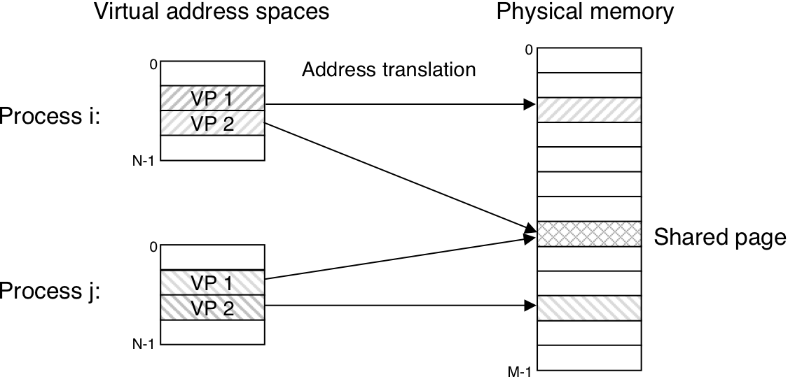
Figure 10.10: The memory image of a Linux process.

Figure 10.11: Using VM to provide page-level memory protection.
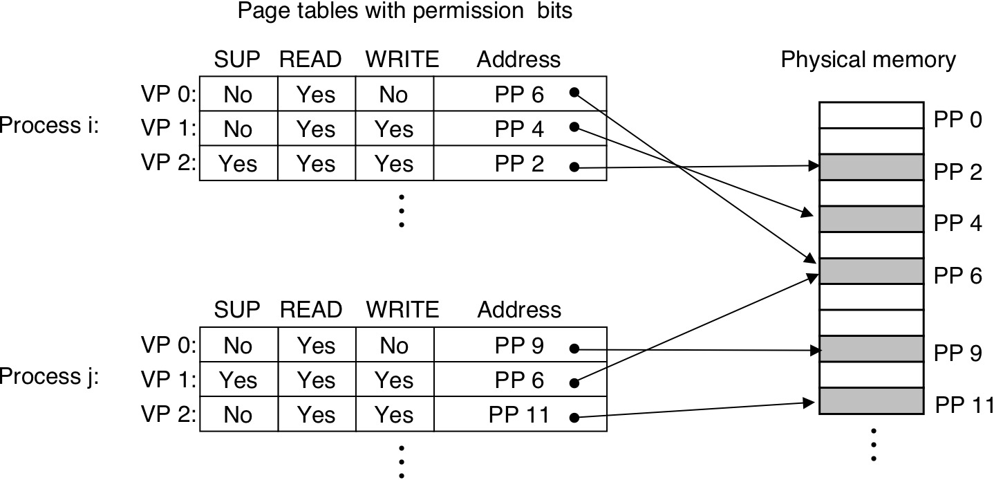
Figure 10.13: Address translation with a page table.
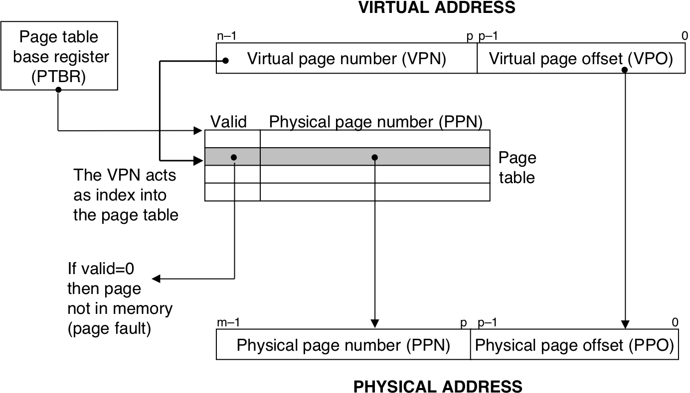
Figure 10.14: Operational view of page hits and page faults.
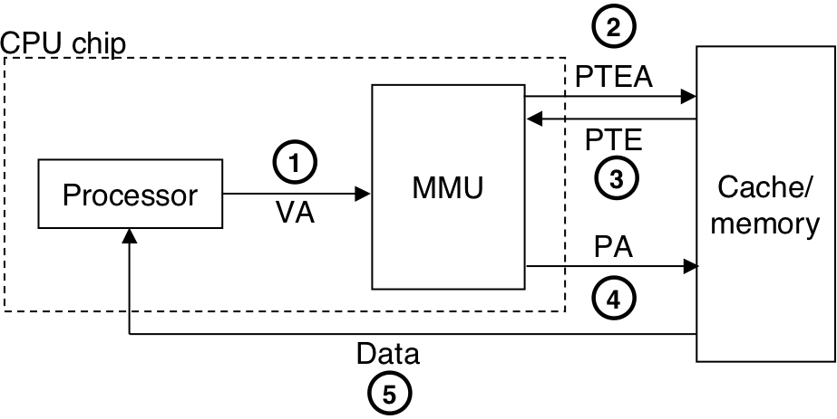
Figure 10.14: Operational view of page hits and page faults.
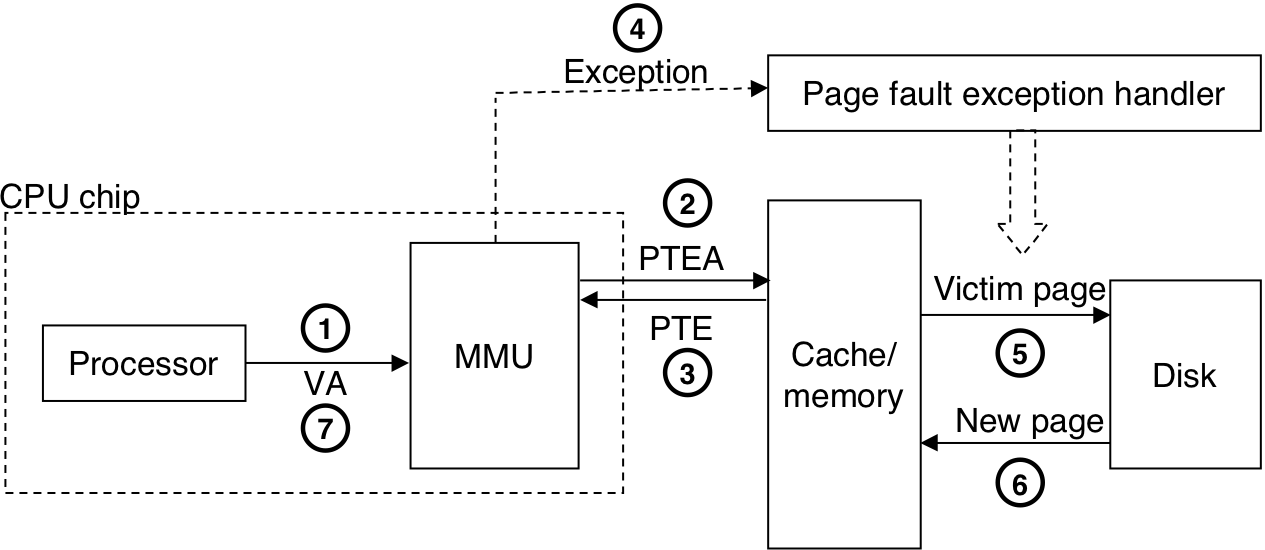
Figure 10.15: Integrating VM with a physically addressed cache.
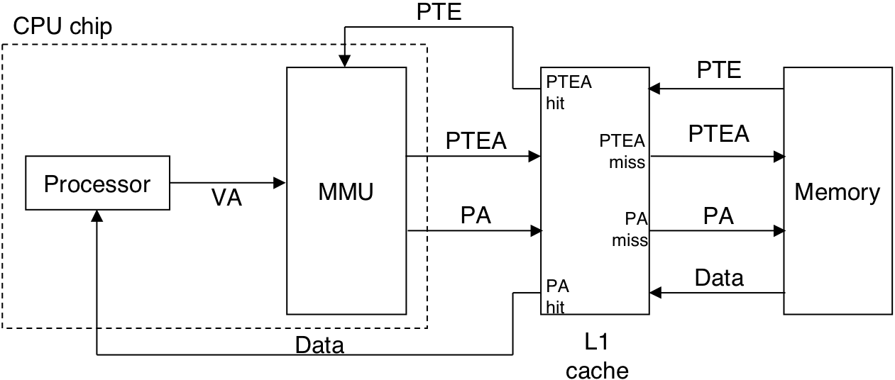
Figure 10.16: Components of a virtual address that are used to access the TLB.
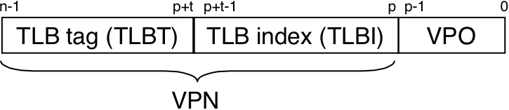
Figure 10.17: Operational view of a TLB hit and miss.
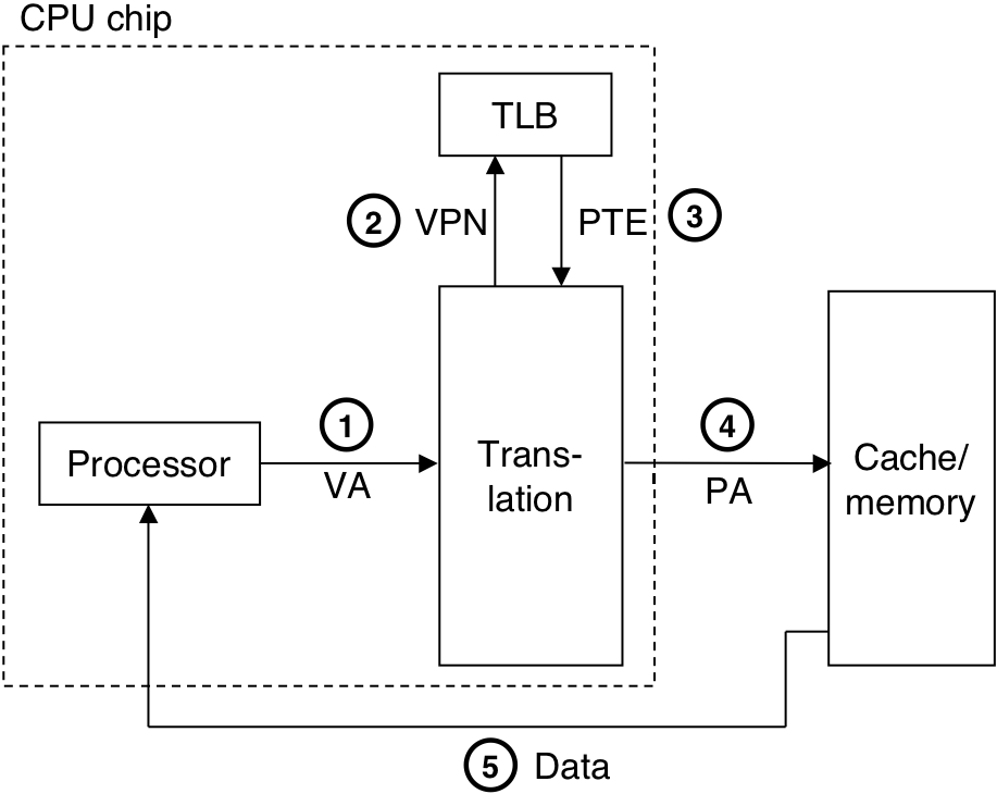
Figure 10.17: Operational view of a TLB hit and miss.
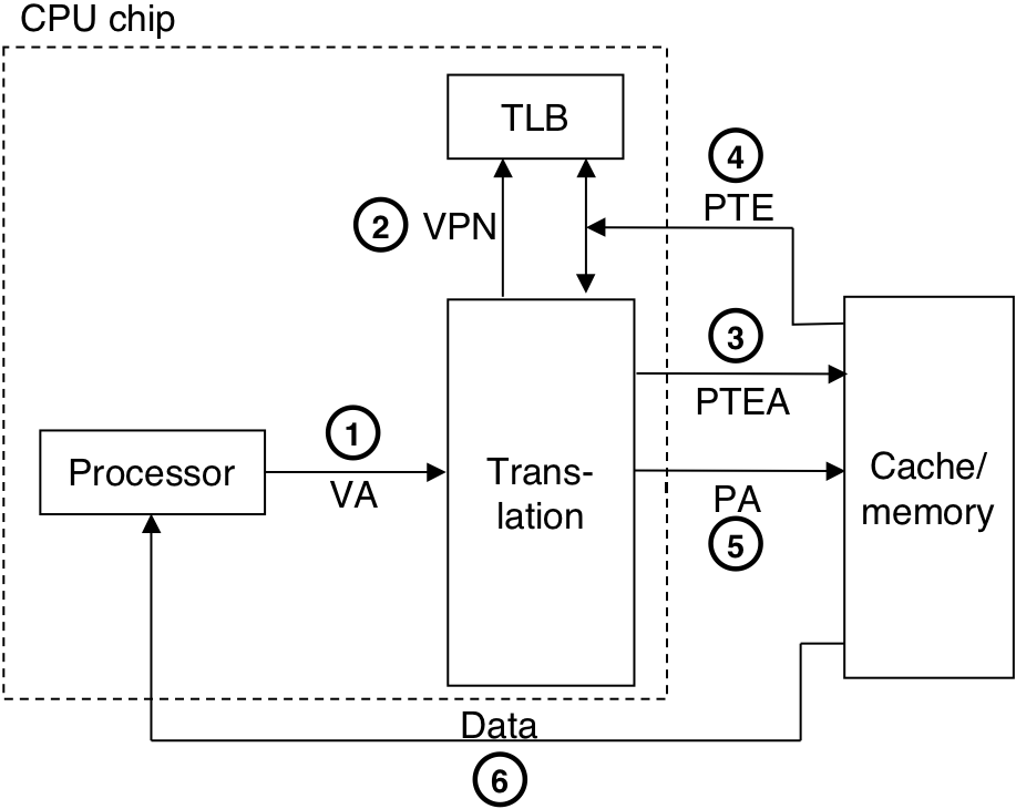
Figure 10.18: A two-level page table hierarchy.
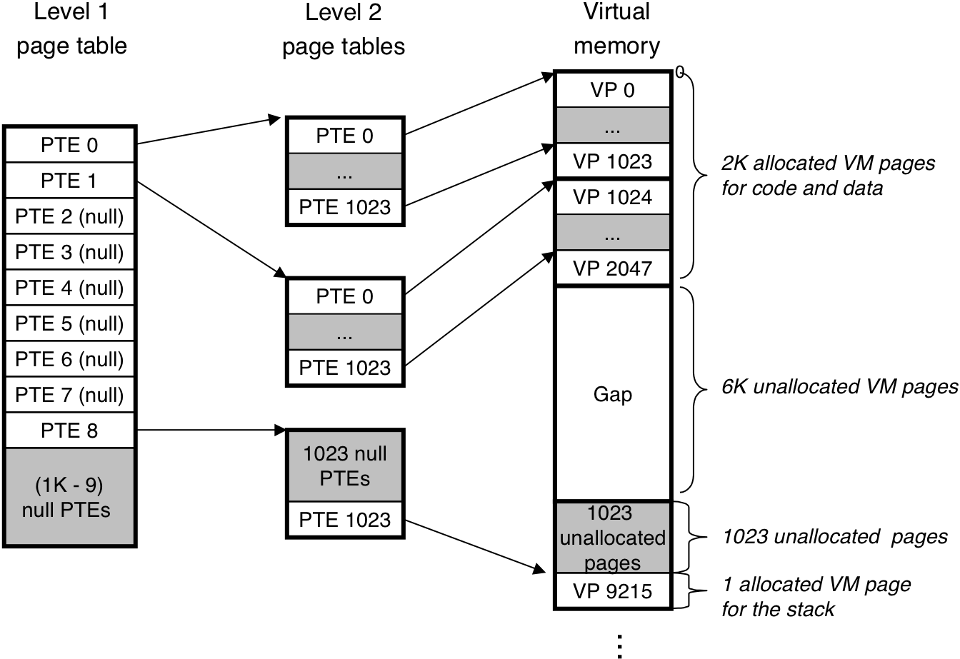
Figure 10.19: Address translation with a k-level page table.
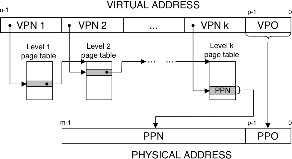
Figure 10.20: Addressing for small memory system.
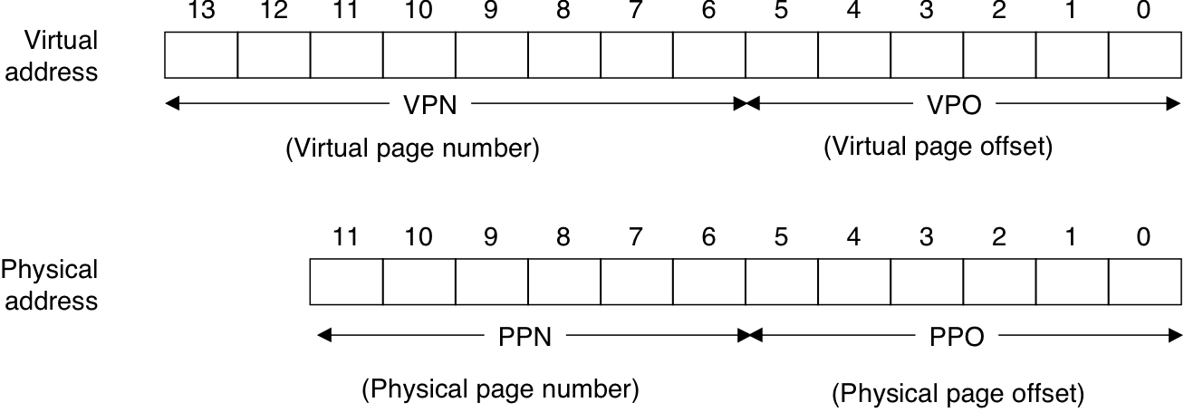
Figure 10.21: TLB, page table, and cache for small memory system.
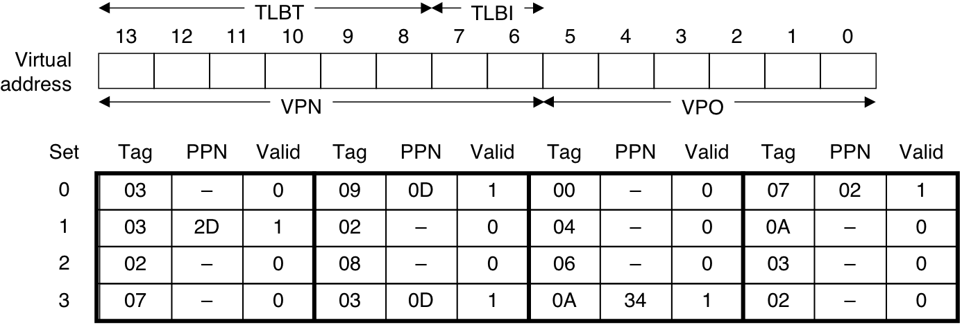
Figure 10.21: TLB, page table, and cache for small memory system.
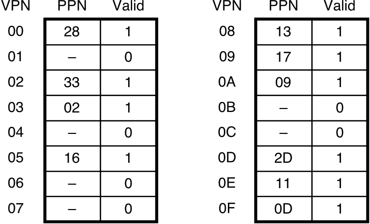
Figure 10.21: TLB, page table, and cache for small memory system.
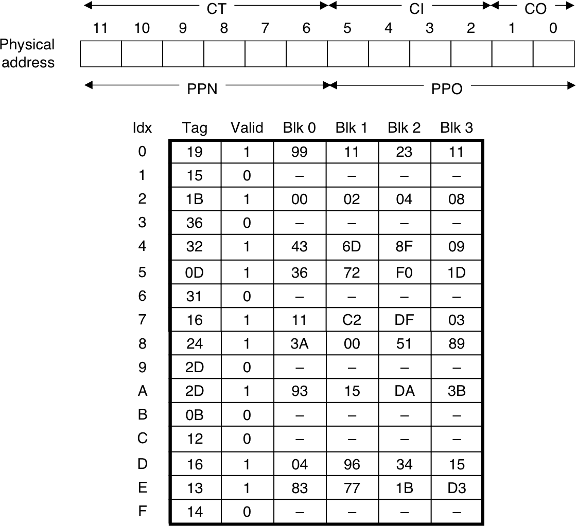
Figure 10.22: The Pentium memory system.
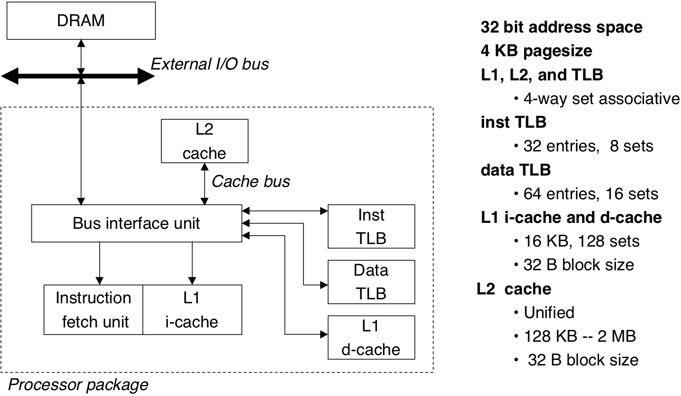
Figure 10.23: Summary of Pentium address translation.
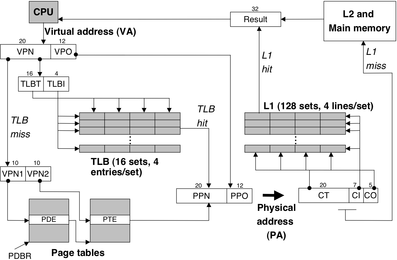
Figure 10.24: Pentium multi level page table.
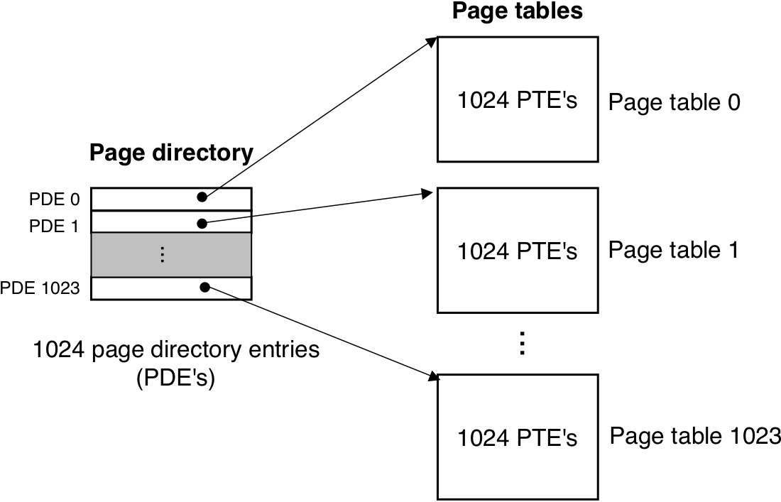
Figure 10.25: Formats of Pentium page directory entry (PDE) and page table entry (PTE).

Figure 10.25: Formats of Pentium page directory entry (PDE) and page table entry (PTE).
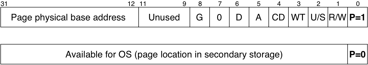
Figure 10.26: Pentium page table translation.
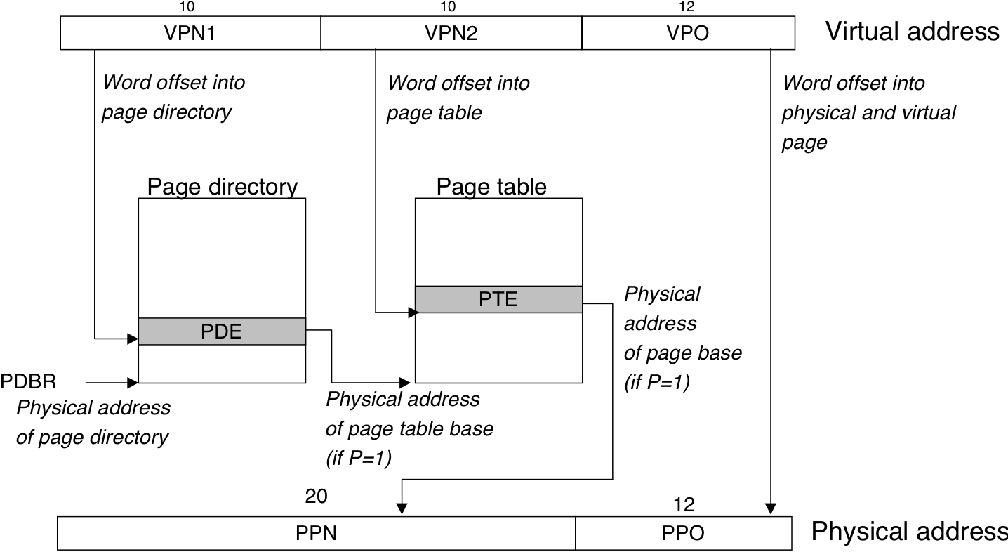
Figure 10.27: Pentium TLB translation.
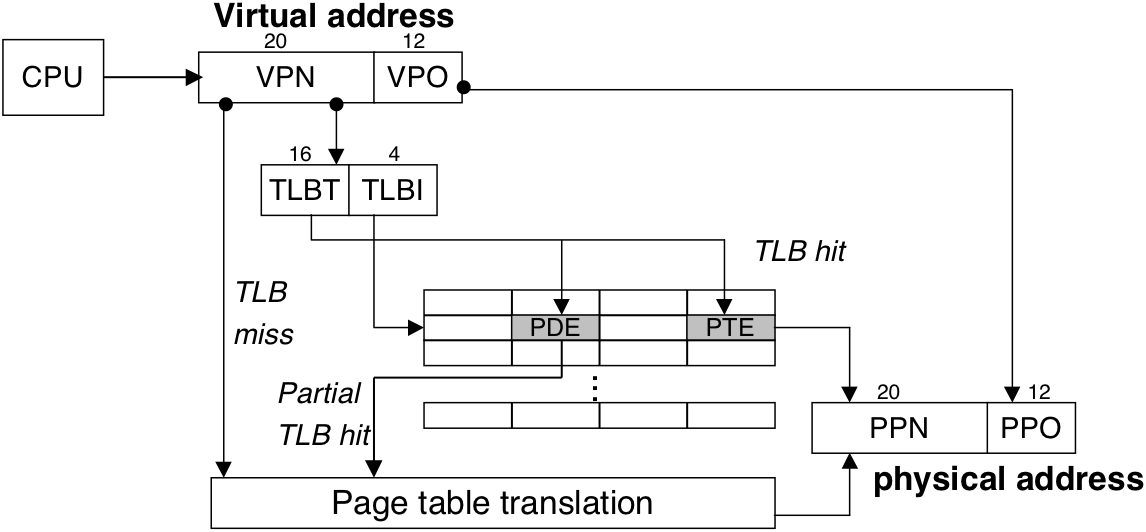
Figure 10.28: The virtual memory of a Linux process.
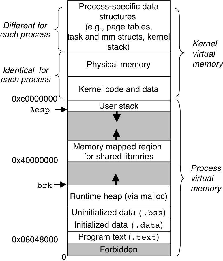
Figure 10.29: How Linux organizes virtual memory.
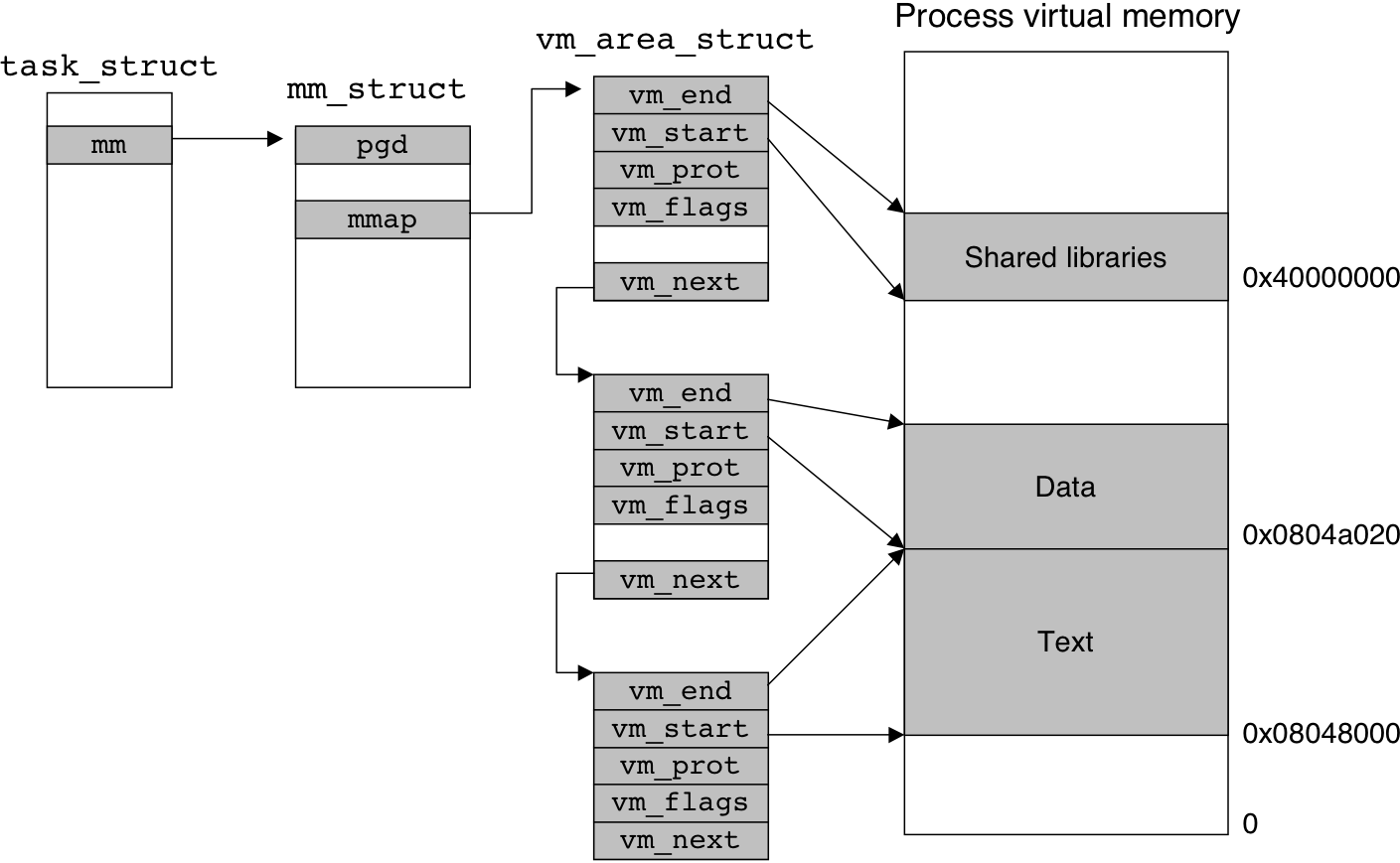
Figure 10.30: Linux page fault handling.
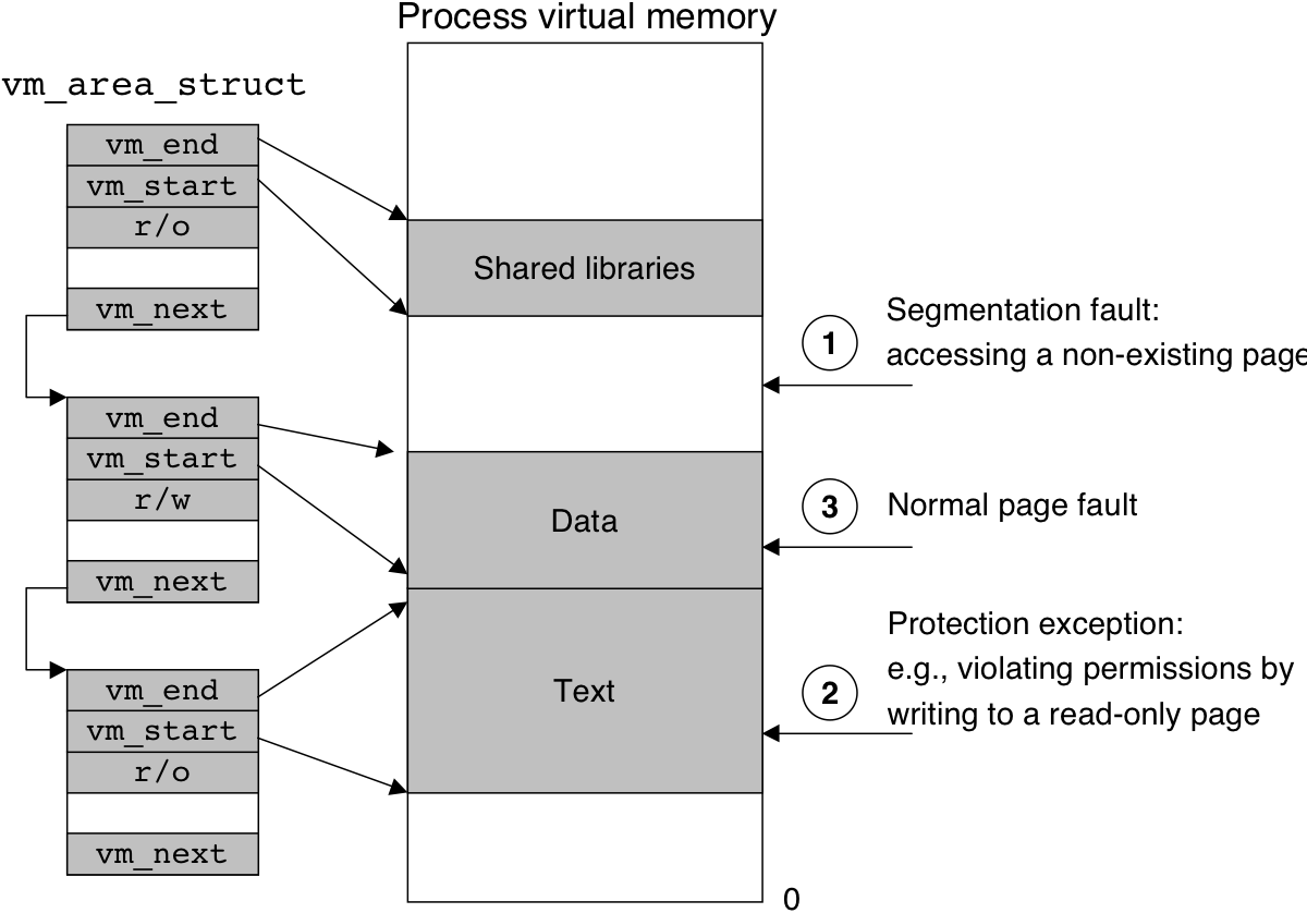
Figure 10.31: A shared object.
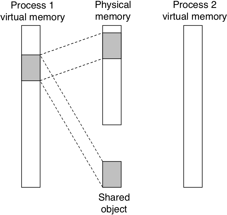
Figure 10.31: A shared object.
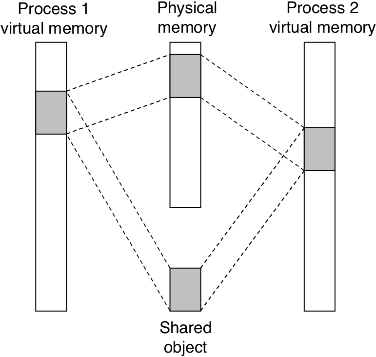
Figure 10.32: A private copy-on-write object.
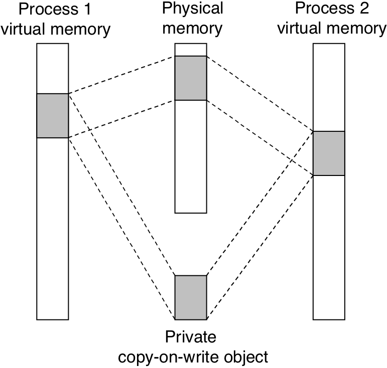
Figure 10.32: A private copy-on-write object.
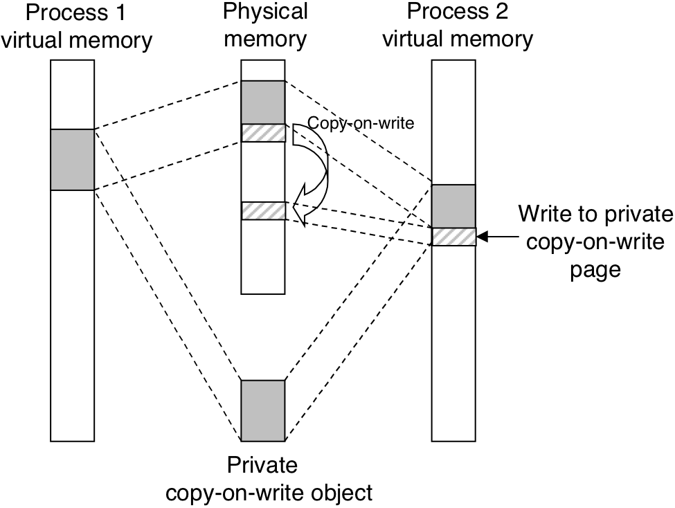
Figure 10.33: How the loader maps the areas of the user address space.
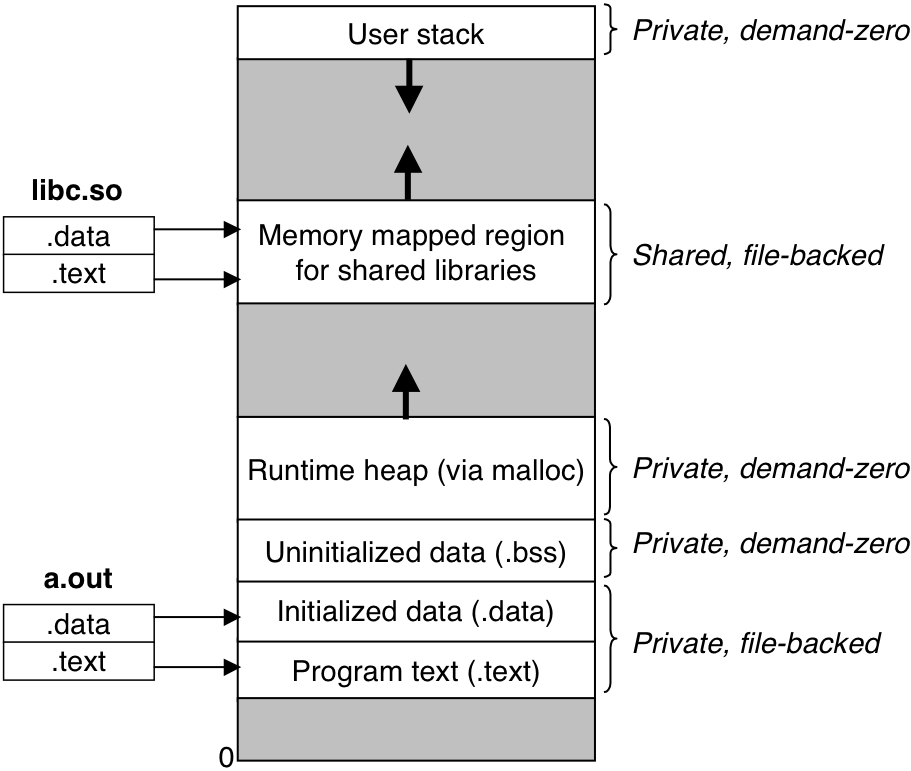
Figure 10.34: Visual interpretation of mmap arguments.
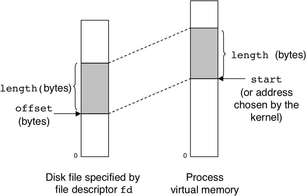
Figure 10.35: The heap.
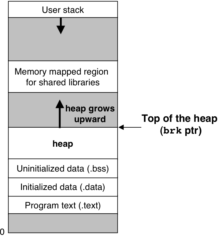
Figure 10.36: Allocating and freeing blocks with malloc.
Figure 10.36: Allocating and freeing blocks with malloc.
Figure 10.36: Allocating and freeing blocks with malloc.
Figure 10.36: Allocating and freeing blocks with malloc.
Figure 10.36: Allocating and freeing blocks with malloc.
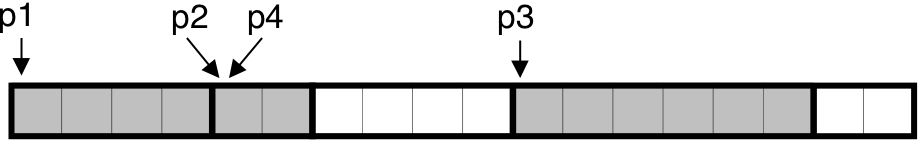
Figure 10.37: Format of a simple heap block.
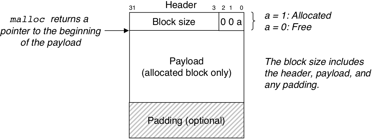
Figure 10.38: Organizing the heap with an implicit free list.
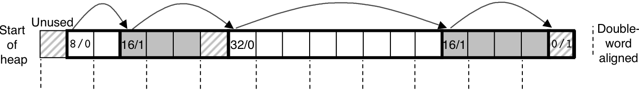
Figure 10.39: Splitting a free block to satisfy a three-word allocation request.
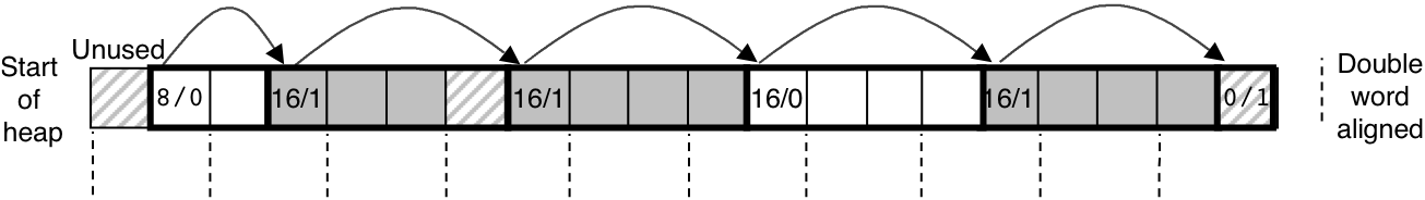
Figure 10.40: An example of false fragmentation.
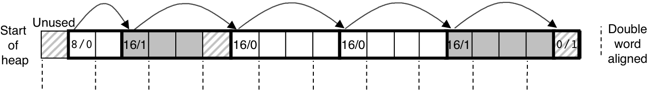
Figure 10.41: Format of heap block that uses a boundary tag.
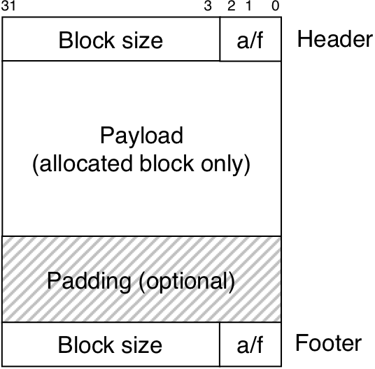
Figure 10.42: Coalescing with boundary tags.
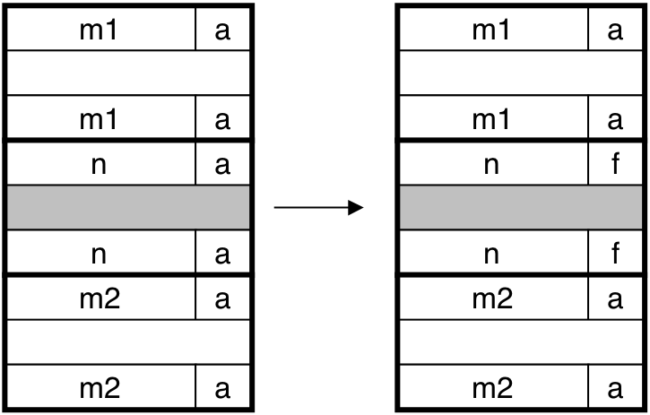
Figure 10.42: Coalescing with boundary tags.
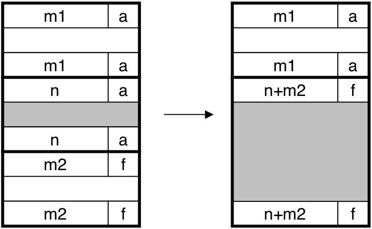
Figure 10.42: Coalescing with boundary tags.
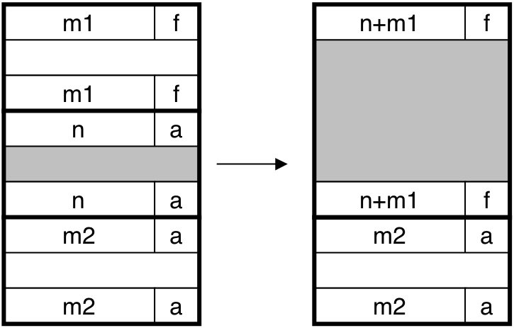
Figure 10.42: Coalescing with boundary tags.
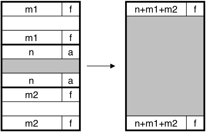
Figure 10.44: Invariant form of the implicit free list.
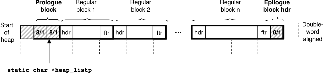
Figure 10.50: Format of heap blocks that use doubly-linked free lists.
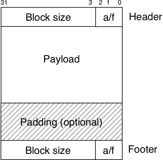
Figure 10.50: Format of heap blocks that use doubly-linked free lists.
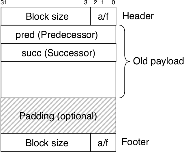
Figure 10.51: A garbage collector's view of memory as a directed graph.
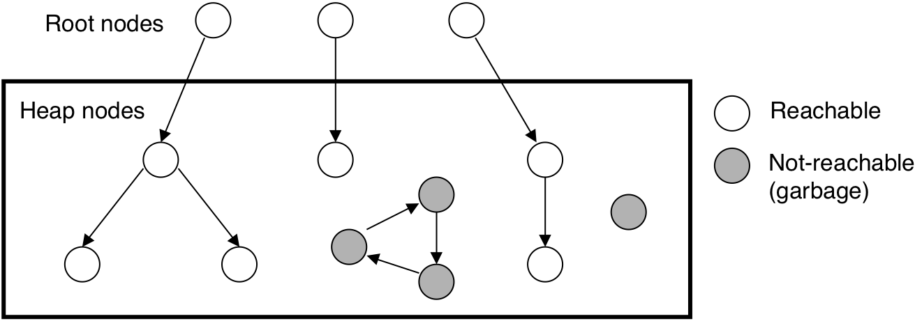
Figure 10.52: Integrating a conservative garbage collector and a C malloc package.
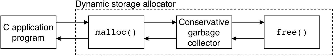
Figure 10.54: Mark and sweep example.
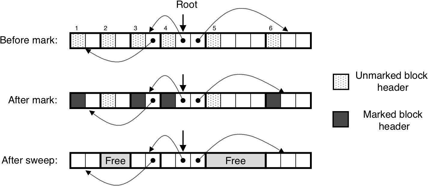
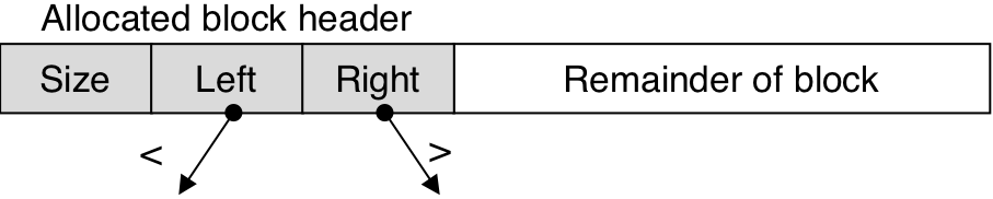
Figure 10.55: Left and right pointers in a balanced tree of allocated blocks.
| 11 [11/13] |
Figure 11.11: Typical kernel data structures for open files.
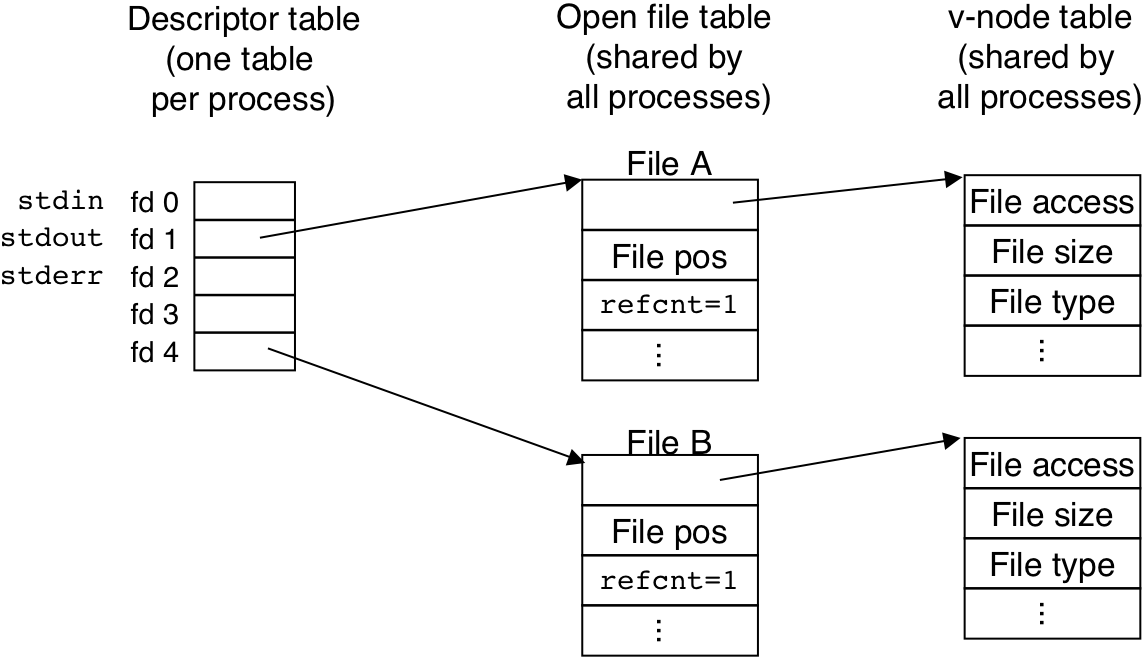
Figure 11.12: File sharing.
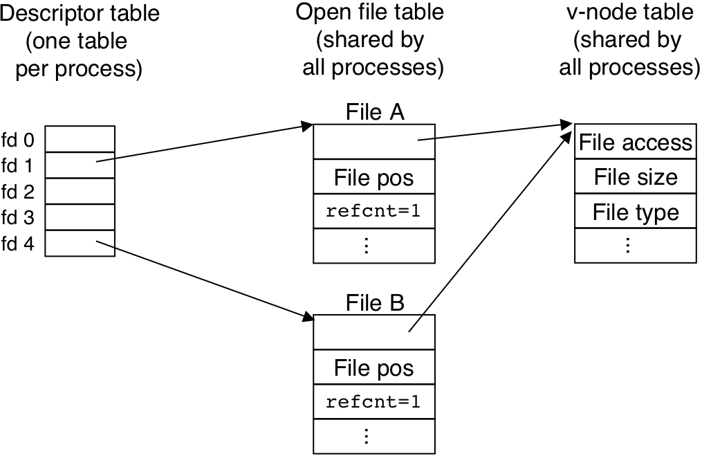
Figure 11.13: How a child process inherits the parent's open files.
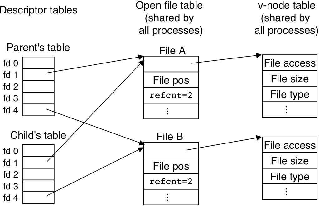
Figure 11.14: Kernel data structures after redirecting standard output by calling dup2(4,1)
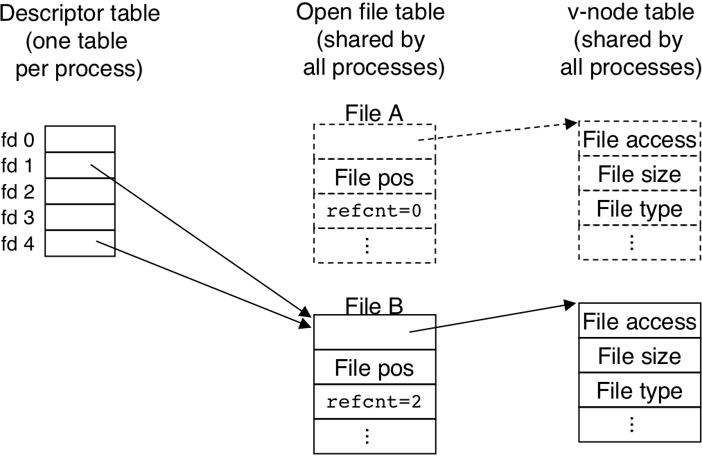
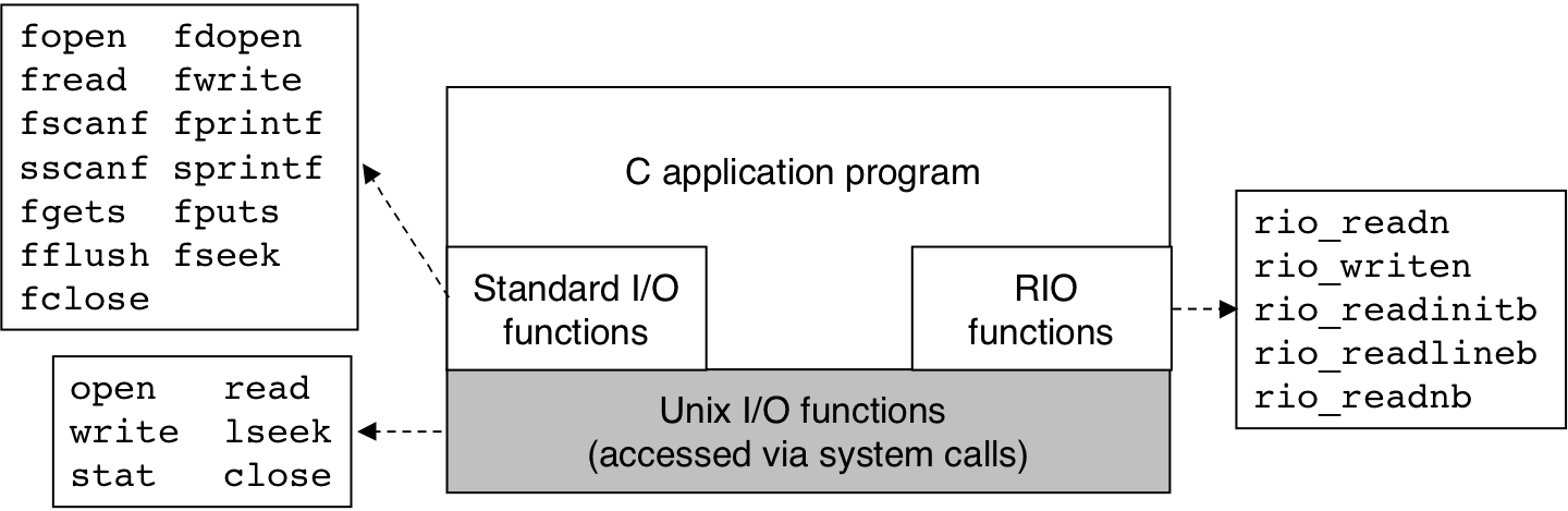
Figure 11.15: Relationship between Unix I/O, standard I/O, and RIO.
| 12 [12/13] |
Figure 12.1: A client-server transaction.
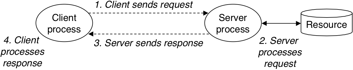
Figure 12.2: Hardware organization of a network host.
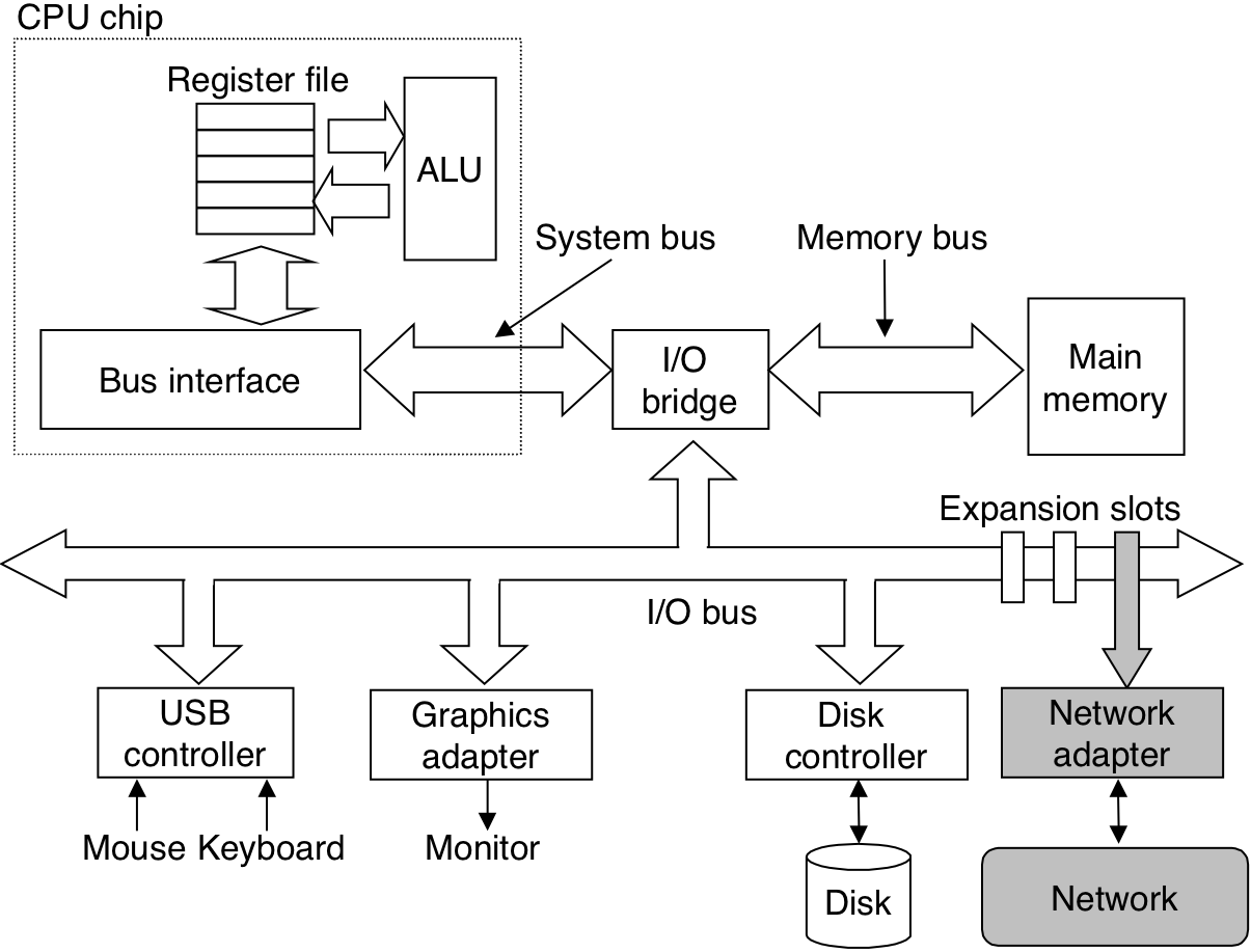
Figure 12.3: Ethernet segment.
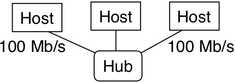
Figure 12.4: Bridged Ethernet segments.
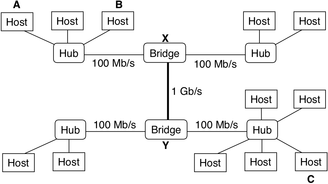
Figure 12.5: Conceptual view of a LAN.
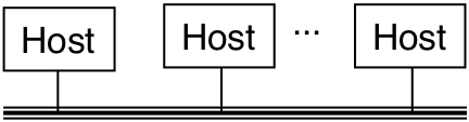
Figure 12.6: A small internet.
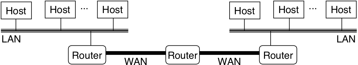
Figure 12.7: How data travels from one host to another on an internet.
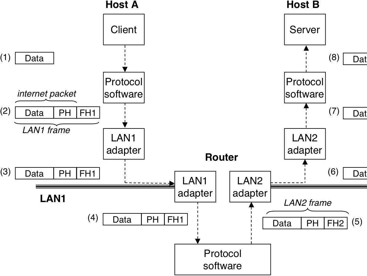
Figure 12.8: Hardware and software organization of an Internet application.
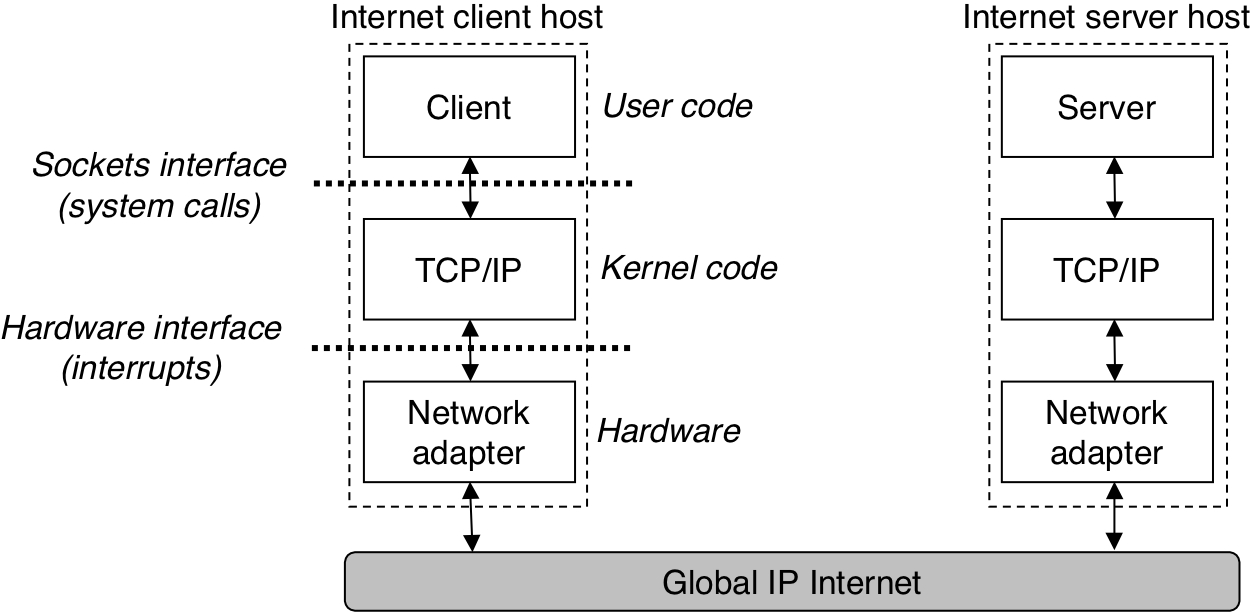
Figure 12.10: Subset of the Internet domain name hierarchy.
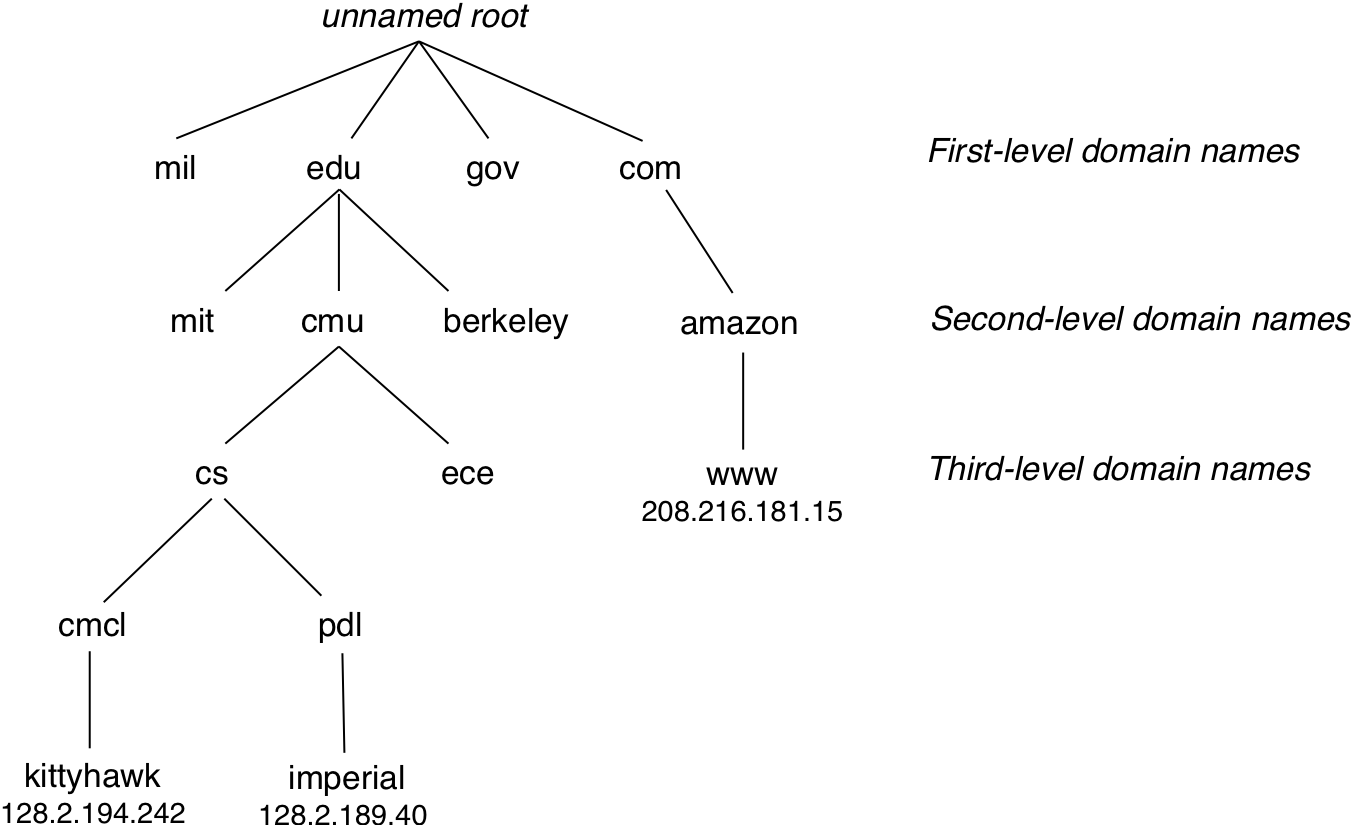
Figure 12.13: Anatomy of an Internet connection
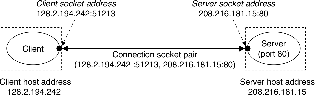
Figure 12.14: Overview of the sockets interface.
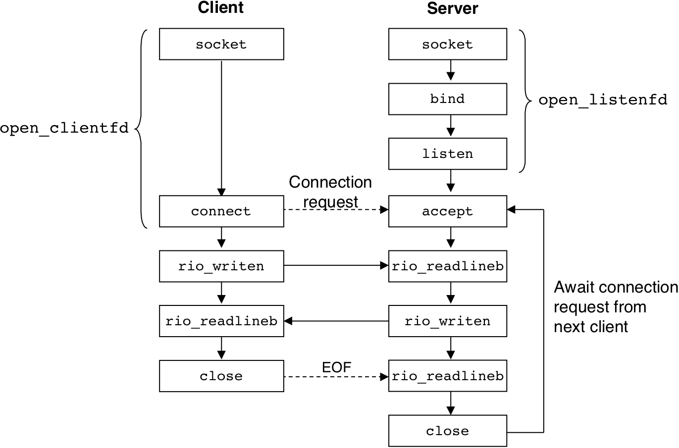
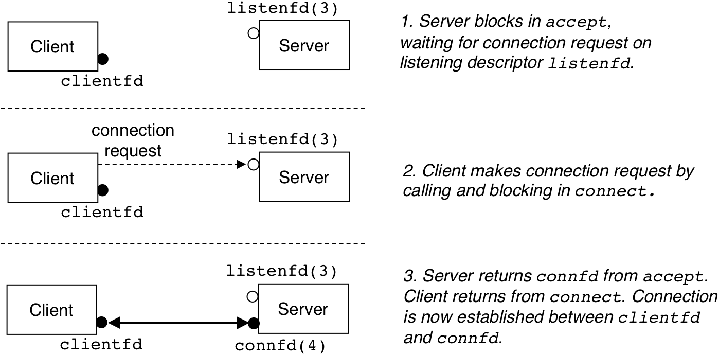
Figure 12.18: The roles of the listening and connected descriptors.
| 13 [13/13] |
Figure 13.1: Step 1: Server accepts connection request from client.
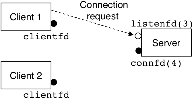
Figure 13.2: Step 2: Server forks a child process to service the client.
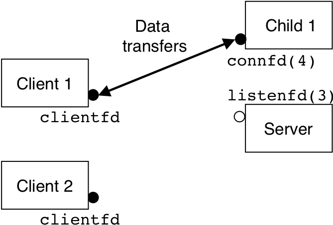
Figure 13.3: Step 3: Server accepts another connection request.
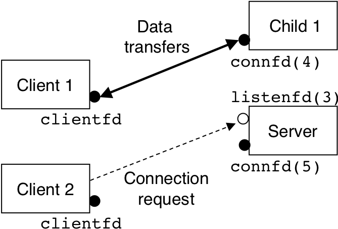
Figure 13.4: Step 4: Server forks another child to service the new client.
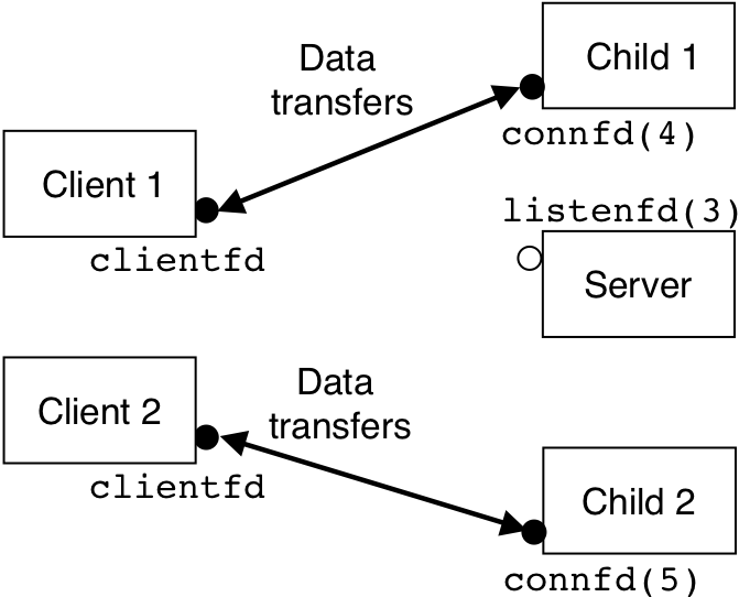
Figure 13.7: State machine for a logical flow in a concurrent event-driven echo server.
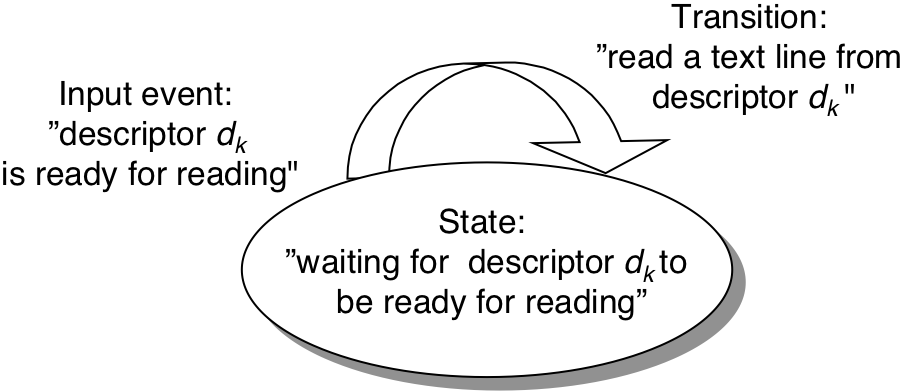
Figure 13.12: Concurrent thread execution.
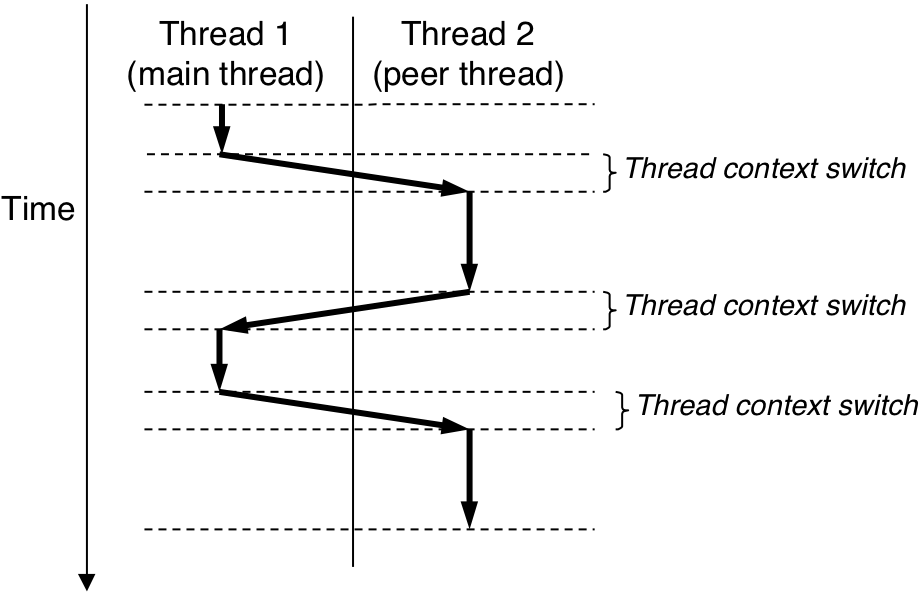
Figure 13.17: IA32 assembly code for the counter loop in badcnt.c.
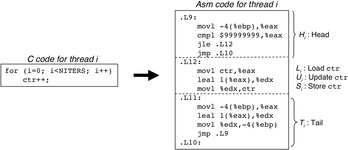
Figure 13.19: Progress graph for the first loop iteration of badcnt.c.
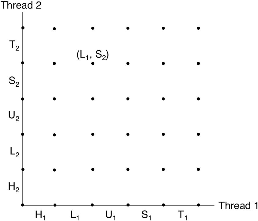
Figure 13.20: An example trajectory.
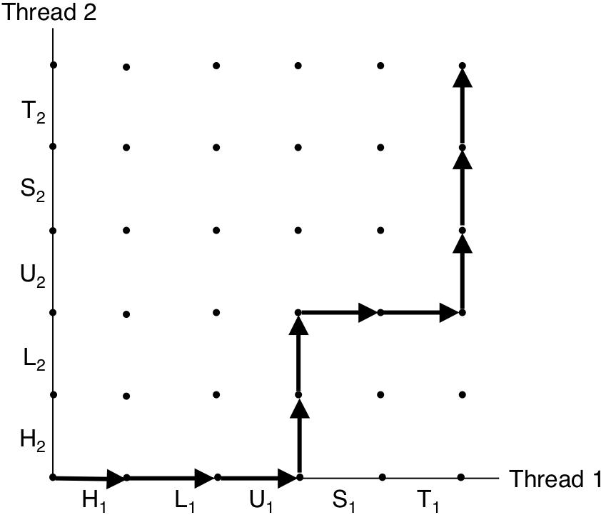
Figure 13.21: Critical sections and unsafe regions.
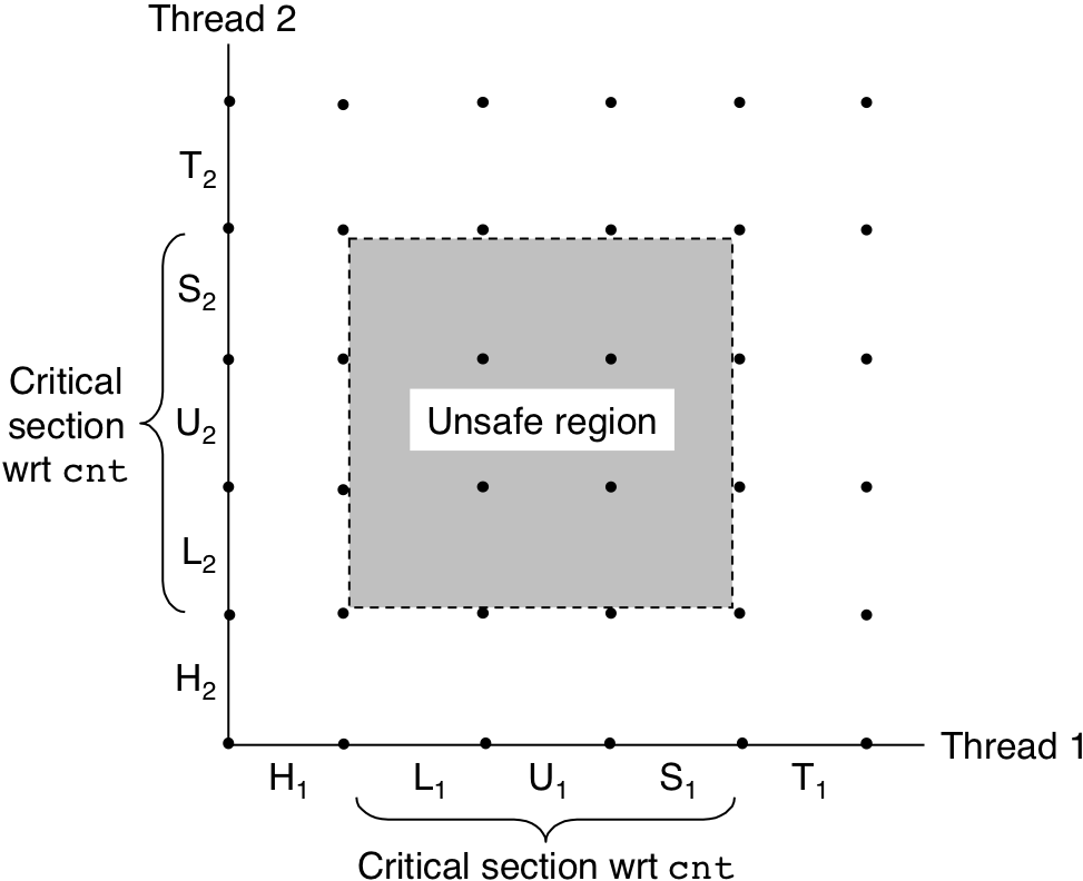
Figure 13.22: Safe and unsafe trajectories.
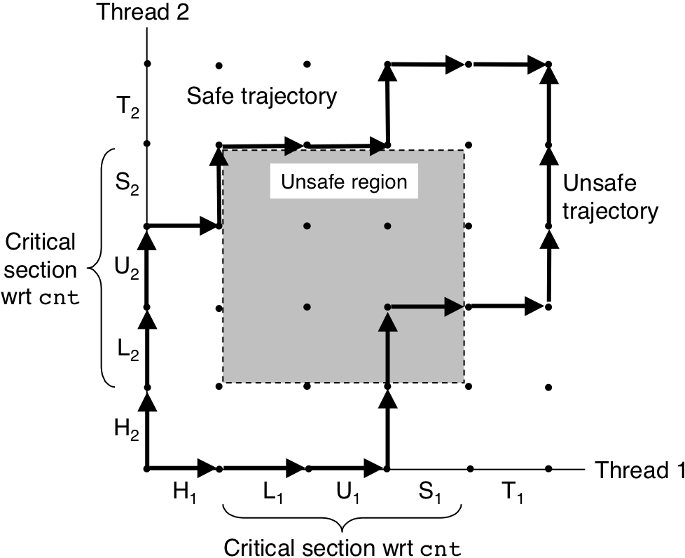
Figure 13.23: Safe sharing with semaphores.
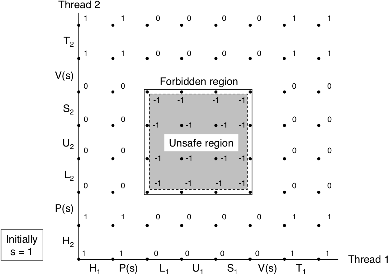
Figure 13.24: Producer-consumer model.
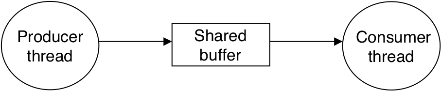
Figure 13.29: Organization of a prethreaded concurrent server.
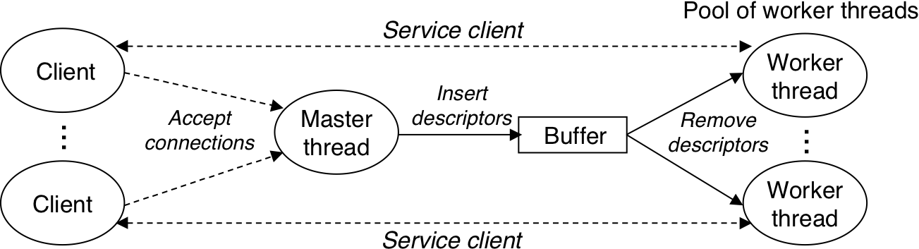
Figure 13.34: Relationships between the sets of reentrant, thread-safe, and nonthread-safe functions.
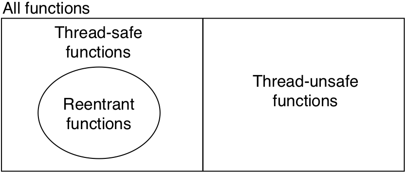
Figure 13.39: Progress graph for a program that can deadlock.
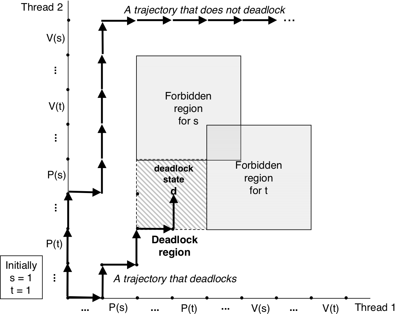
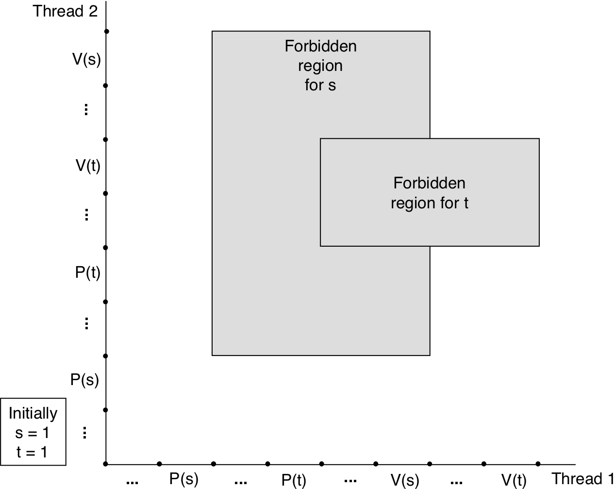
Figure 13.40: Progress graph for a deadlock-free program.
Revised: 2007/04/05 17:41